Code
import numpy as np
import matplotlib.pyplot as plt
from IPython.display import display, Markdown
import sympy as sp⏱ 2h, déposer le notebook dans Moodle (si 1/3 temps supplémentaire, 2h40)
📚 Autorisés : notebooks de cours, notes personnelles.
Compléter ici :
Déterminer les coefficients d’un schéma multi-pas linéaire explicite à deux pas sous les conditions suivantes :
Considérer le problème de Cauchy suivant : \( \begin{cases} y'(t) = \frac{y^2(t)}{t}, & t \in [1, t_{\text{max}}], \\ y(1) = 2. & \end{cases} \) Déterminer \(t_{\text{max}}\). (Suggéstion : calculer la solution exacte de ce problème de Cauchy).
Implémenter le schéma déterminé à la question 1 pour résoudre le problème de Cauchy. Vérifier expérimentalement l’ordre de convergence du schéma sur l’intervalle \([1, \frac{1 + t_{\text{max}}}{2}]\).
Correction
Un schéma multi-pas linéaire explicite à \(q=2\) pas s’écrit comme
\( u_{n+1} = a_0 u_n + a_1 u_{n-1} + h \Big( b_0 \varphi_n + b_1 \varphi_{n-1} \Big). \)
Le premier polynomial caractéristique est donné par
\( \varrho(r) = r^2 - a_0 r - a_1. \)
Le schéma est convergent, ainsi \(r=1\) est une racine. On sait aussi que \(r=\frac{1}{6}\) est une racine, donc
\( \varrho(r) = (r-1)\left(r-\frac{1}{6}\right) = r^2 - \frac{7}{6} r + \frac{1}{6}. \)
Par identification des coefficients, on trouve \(a_0=\frac{7}{6}\) et \(a_1=-\frac{1}{6}\).
Il ne reste qu’à trouver les coefficients \(b_0\) et \(b_1\). Le schéma est convergent à l’ordre au moins 2 ssi \(\xi(0)=\xi(1)=\xi(2)=1\). La condition \(\xi(0)=1\) est déjà satisfaite car \(r=1\) est une racine du polynôme caractéristique. On a alors les deux équations
\( \(\begin{cases} -a_1+b_0+b_1 = 1\\ a_{1} - 2 b_{1} = 1 \end{cases}\)\(\begin{cases} \frac{1}{6}+b_0+b_1 = 1\\ -\frac{1}{6} - 2 b_{1} = 1 \end{cases}\) \(\begin{cases} b_0 = \frac{17}{12}\\ b_1 = -\frac{7}{12} \end{cases}\)
\)
Conclusion : un seul schéma satisfait à toutes les conditions, il s’agit du schéma
\( u_{n+1} = \frac{7}{6} u_n - \frac{1}{6} u_{n-1} + \frac{h}{12} \left( 17 \varphi_n - 7 \varphi_{n-1} \right). \)
import numpy as np
import matplotlib.pyplot as plt
from IPython.display import display, Markdown
import sympy as sp# Vérifions nos calculs avec sympy
# ================================
a0, a1 = sp.symbols('a0 a1')
b0, b1 = sp.symbols('b0 b1')
r = sp.symbols('r')
Eq0 = sp.Eq( (r-1)*(r-1/sp.S(6)) , r**2 - a0*r-a1 )
aa = sp.solve(Eq0, (a0,a1))
for k,v in aa.items():
display(sp.Eq(k,v))
a0 = aa[a0]
a1 = aa[a1]
Eq1 = sp.Eq(-a1 + b0+ b1, 1)
Eq2 = sp.Eq(a1 -2* b1, 1)
sol = sp.solve((Eq1, Eq2), (b0, b1))
for k,v in sol.items():
display(sp.Eq(k,v))\(\displaystyle a_{0} = \frac{7}{6}\)
\(\displaystyle a_{1} = - \frac{1}{6}\)
\(\displaystyle b_{0} = \frac{17}{12}\)
\(\displaystyle b_{1} = - \frac{7}{12}\)
Calculons la solution exacte du problème de Cauchy. L’EDO est à variables séparables : \(\frac{dy}{y^2} = \frac{dt}{t}\). En intègrant de chaque côté on trouve \(-\frac{1}{y} = \ln|t| + C\). Avec \(y(1) = 2\) on trouve la constante d’intégration : \(-\frac{1}{2} = \ln(1) + C \leadsto C = -\frac{1}{2}\). Donc \(y(t) = \frac{1}{\frac{1}{2} - \ln(t)}\).
La solution exacte du problème de Cauchy est donnée par \(y(t) = \frac{2}{1-2\log(t)}\) qui n’est pas définie en \(t=\sqrt{e}\). Ainsi, \(t_{\text{max}} = \sqrt{e}\).
# ==================================================
# TEST
# ==================================================

phi = lambda t,y : y**2/t
t0, y0 = 1, 2


# Solution exacte
# ---------------
t = sp.symbols('t')
y = sp.Function('y')(t)
eq = sp.Eq(y.diff(t), phi(t, y))
display(eq)
ics = {y.subs(t, t0): y0 }
display(sp.Eq(y.subs(t, t0), y0))
sol = sp.dsolve(eq, y, ics=ics)
display(Markdown(f"La solution exacte est"))
display(sol)

display(Markdown(r"On en déduit que $t < \sqrt{e}$"))

# Transfomation en fonction numpy
# -------------------------------

sol = sp.lambdify(t, sol.rhs, 'numpy')
tfin = (t0+np.sqrt(np.exp(1)))/2
\(\displaystyle \frac{d}{d t} y{\left(t \right)} = \frac{y^{2}{\left(t \right)}}{t}\)
\(\displaystyle y{\left(1 \right)} = 2\)
La solution exacte est
\(\displaystyle y{\left(t \right)} = - \frac{1}{\log{\left(t \right)} - \frac{1}{2}}\)
On en déduit que \(t < \sqrt{e}\)
def MPL(phi, tt, sol_exacte) :
    uu = np.zeros_like(tt)
    h = tt[1]-tt[0]
    q = 2
    uu[:q] = sol_exacte(tt[:q])
    for n in range(q-1, len(tt)-1) :
        k0 = phi(tt[n], uu[n])
        k1 = phi(tt[n-1], uu[n-1])
        uu[n+1] = (7*uu[n]-uu[n-1])/6 + h*(17*k0-7*k1)/12
    return uu


# Solution numérique : vérification de l'implémentation
# -----------------------------------------------------
# tt = np.linspace(t0, tfin, 100)
# uu = MPL(phi, tt, sol)
# plt.plot(tt, uu, label='MPL')
# plt.plot(tt, sol(tt), label='Solution exacte')
# plt.legend();

# Calcul de l'ordre de convergence
# --------------------------------

H, err = [], []
for N in range(50,500,50) :
    tt = np.linspace(t0, tfin, N)
    uu = MPL(phi, tt, sol)
    err.append(np.linalg.norm(uu-sol(tt), np.inf))
    H.append(tt[1]-tt[0])

pente = np.polyfit(np.log(H), np.log(err), 1)[0]
plt.loglog(H, err, 'o-')
plt.title(f"{pente = }")
plt.xlabel('h')
plt.ylabel('Erreur');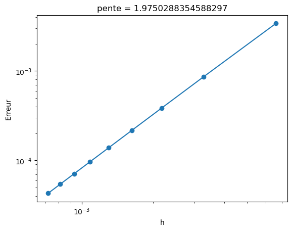
On considère le schéma de Runge-Kutta explicite à 3 étages défini par le tableau de Butcher suivant :
\( \begin{array}{c|ccc} 0 & 0 & 0 & 0 \\ 1/2 & 1/2 & 0 & 0 \\ 1 & -1 & 2 & 0 \\ \hline & 1/6 & 2/3 & 1/6 \end{array} \)
On considère le problème de Cauchy \(y'(t) = -\beta y(t)\) et \(y(0) = 1\) avec \(\beta>0\).
Le schéma est donné par
\( \begin{aligned} k_1 &= \varphi\Big(t_n, u_n\Big) \\ k_2 &= \varphi\Big(t_n + \frac{1}{2}h, u_n + \frac{1}{2}hk_1\Big) \\ k_3 &= \varphi\Big(t_n + h, u_n + h(-k_1 + 2k_2) \Big) \\ u_{n+1} &= u_n + \frac{1}{6}h\Big(k_1 + 4k_2 + k_3\Big) \end{aligned} \)
On applique le schéma au problème de Cauchy \(y'(t) = -\beta y(t)\) et \(y(0) = 1\) avec \(\beta>0\) dont la solution est \(y(t)=e^{-\beta t}\). Avec \(\varphi(t, y) = -\beta y\), on obtient alors la relation de récurrence suivante :
\( \begin{aligned} k_1 &= -\beta u_n \\ k_2 &= -\beta\Big(u_n + \frac{1}{2}hk_1\Big) = -\Big(1 - \frac{1}{2}\beta h\Big)\beta u_n \\ k_3 &= -\beta\Big(u_n + h(-k_1 + 2k_2) \Big) = -\Big(\beta^2 h^2 - \beta h + 1\Big)\beta u_n \\ u_{n+1} &= u_n + \frac{1}{6}h\Big(k_1 + 4k_2 + k_3\Big) = -\frac{(\beta h)^3}{6} + \frac{(\beta h)^2}{2} -(\beta h)+1 \end{aligned} \)
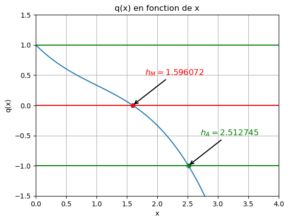
On notera \(x = \beta h>0\) et \(q(x)\) le facteur d’amplification du schéma :
\( q(x) = \frac{u_{n+1}}{u_n} = -\frac{x^3}{6} + \frac{x^2}{2} -x+1 \)
La suite vérifie \(u_n \xrightarrow[n\to \infty]{} 0\) ssi \(\left|q(x)\right|<1\). En étudiant brièvement la fonction \(q(x)\), on trouve que \(q\) est une fonction monotone décroissante avec \(q(0)=1\) et \(q(x)\xrightarrow[x\to+\infty]{}-\infty\). On cherche alors les solutions de \(q(x)+1=0\).
Il n’est pas possible de résoudre analytiquement cette équation, on utilisera donc fsolve pour déterminer une valeur approchée de \(x\) pour laquelle le schéma est A-stable.
De même, le schéma génère une solution monotone ssi \(q(x)>0\) . On cherche alors numériquement les solutions de \(q(x)=0\).
from IPython.display import display, Markdown
import numpy as np
import matplotlib.pyplot as plt
from scipy.optimize import fsolve

q_func = lambda x: -x**3/6+x**2/2-x+1

x = np.linspace(0,4,101)
plt.plot(x, q_func(x))
plt.hlines(1,0,4, color='green')
plt.hlines(-1,0,4, color='green')
plt.hlines(0,0,4, color='red')
plt.ylim(-1.5,1.5)
plt.xlim(0,4)
plt.grid()
plt.xlabel('x')
plt.ylabel('q(x)')
plt.title('q(x) en fonction de x')

h_A = fsolve(lambda x: q_func(x)+1, 2)[0]
h_M = fsolve(lambda x: q_func(x), 1)[0]

plt.scatter(h_A, -1, color='green')
plt.annotate(f'$h_A = {h_A:.6f}$', xy=(h_A, -1), xytext=(h_A+0.2, -0.5), arrowprops=dict(arrowstyle='->', lw=1.5), fontsize=12, color='green')
plt.scatter(h_M, 0, color='red')
plt.annotate(f'$h_M = {h_M:.6f}$', xy=(h_M, 0), xytext=(h_M+0.2, 0.5), arrowprops=dict(arrowstyle='->', lw=1.5), fontsize=12, color='red')

display(Markdown(f"La condition de A-stabilité est satisfaite pour $\\beta h < {h_A:.6f}$"))
display(Markdown(f"La condition de monotonie est satisfaite pour $\\beta h < {h_M:.6f}$"))
La condition de A-stabilité est satisfaite pour \(\beta h < 2.512745\)
La condition de monotonie est satisfaite pour \(\beta h < 1.596072\)
On peut vérifier nos calculs avec sympy :
import sympy as sp

b = [1/sp.S(6), 2/sp.S(3), 1/sp.S(6)]
c = [0,1/sp.S(2),1]
A = [[0, 0, 0], [1/sp.S(2), 0, 0], [-1, 2, 0]]

s = len(c)

u_n = sp.symbols(r'u_n')
u_np1 = sp.symbols(r'u_{n+1}')

dt = sp.symbols(r'h', positive=True)
x = sp.symbols(r'x', positive=True)

k_1 = sp.symbols(r'k_1')
k_2 = sp.symbols(r'k_2')
k_3 = sp.symbols(r'k_3')
kk = [k_1, k_2, k_3]

beta = sp.symbols(r'\beta', positive=True)
phi = lambda y: -beta*y

display(Markdown("**Les équations**"))
Eqs = [ sp.Eq(kk[i] ,  phi(u_n + dt*sum([kk[j]*A[i][j] for j in range(s)]))) for i in range(s) ]
for eq in Eqs:
    display(eq)

display(Markdown("**Ce qui donne**"))
sol = sp.solve( Eqs, kk ) # c'est un dictionnaire
KK = [sol[kk[i]] for i in range(s)]
for i,k in enumerate(KK):
    display(sp.Eq(kk[i]/u_n, k.factor()/u_n))

display(Markdown("**Enfin**"))
schema = sp.Eq( u_np1/u_n , (u_n + dt*sum([KK[j]*b[j] for j in range(s)])).factor()/u_n )
display(schema)


display(Markdown("**Le facteur d'amplification**"))
q = (schema.rhs).simplify().subs(beta*dt,x)
q_func = sp.lambdify(x, q, modules=['numpy'])
display(sp.Eq(sp.Symbol('q(x)'), q.factor()))

# sp.plot(q, (x,0,10), ylim=(-1.5,1.5),
#             ylabel='$q(x)$', xlabel='$x$')

# # sp.solve(abs(q)<1, x)
display(Markdown(f"La **condition de A-stabilité** est satisfaite pour $\\beta h < {sp.nsolve(abs(q)-1, x, 2):.6f}$"))
display(Markdown(f"La **condition de monotonie** est satisfaite pour $\\beta h < {sp.nsolve(abs(q), x, 2):.6f}$"))
Les équations
\(\displaystyle k_{1} = - \beta u_{n}\)
\(\displaystyle k_{2} = - \beta \left(\frac{h k_{1}}{2} + u_{n}\right)\)
\(\displaystyle k_{3} = - \beta \left(h \left(- k_{1} + 2 k_{2}\right) + u_{n}\right)\)
Ce qui donne
\(\displaystyle \frac{k_{1}}{u_{n}} = - \beta\)
\(\displaystyle \frac{k_{2}}{u_{n}} = \frac{\beta \left(\beta h - 2\right)}{2}\)
\(\displaystyle \frac{k_{3}}{u_{n}} = - \beta \left(\beta^{2} h^{2} - \beta h + 1\right)\)
Enfin
\(\displaystyle \frac{u_{n+1}}{u_{n}} = - \frac{\beta^{3} h^{3}}{6} + \frac{\beta^{2} h^{2}}{2} - \beta h + 1\)
Le facteur d’amplification
\(\displaystyle q(x) = - \frac{x^{3} - 3 x^{2} + 6 x - 6}{6}\)
La condition de A-stabilité est satisfaite pour \(\beta h < 2.512745\)
La condition de monotonie est satisfaite pour \(\beta h < 1.596072\)
Vérifions empiriquement la stabilité du schéma pour \(\beta = 1\).
def RK(phi, tt, yy):
    h = tt[1] - tt[0]
    uu = np.zeros_like(tt)
    uu[0] = yy[0]
    for n in range(len(tt)-1):
        k1 = phi(tt[n], uu[n])
        k2 = phi(tt[n] + h/2, uu[n] + h/2*k1)
        k3 = phi(tt[n] + h, uu[n] - h*k1 + 2*h*k2)
        uu[n+1] = uu[n] + h*(k1 + 4*k2 + k3)/6
    return uu


sol_exacte = lambda t: np.exp(-t)
phi = lambda t, y: -y

tt_M = np.arange(0, 25, h_M/2)
yy_M = sol_exacte(tt_M)
uu_M = RK(phi, tt_M, yy_M)

plt.plot(tt_M, uu_M, '^:', label='RK', lw=2)
plt.plot(tt_M, yy_M, 'o--', label='Solution exacte', lw=3)
plt.legend()
plt.show()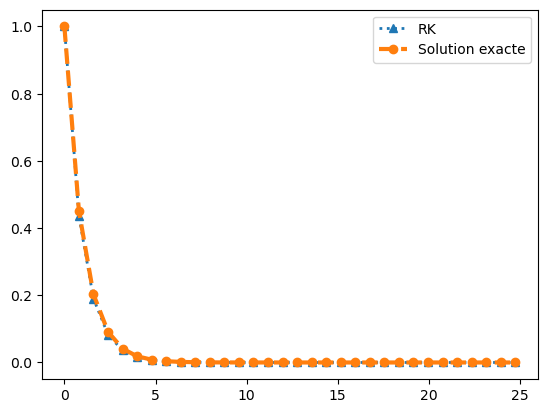
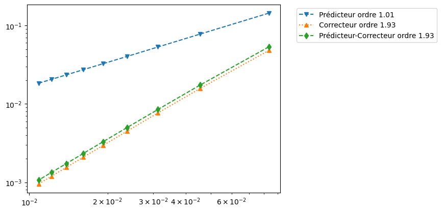
PRED, CORR et PRED_CORR prénant en entrée les paramètres suivants :
phi : la fonction \(\varphi\) du problème de Cauchytt : le vecteur des instants d’évaluationyy : le vecteur des valeurs de la solution exacte aux temps \(t_0\) et \(t_1\)uu le vecteur des valeurs de la solution approchée aux instants d’évaluation tt.\( \begin{cases} y'(t) = \arctan(5(1-t))y(t) \quad \text{pour } t \in ]0,3] \\ y(0) = \sqrt[10]{26} \end{cases} \)
Correction
Le schéma PC est donné par
\( \begin{cases} u_0 = y_0 \\ u_1 = y_1 \\ \tilde u_{n+1} = u_n + h\varphi(t_n, u_n) \\ u_{n+1} = \frac{1}{3}\Big(4 u_{n} - u_{n-1} + 2h\varphi(t_{n+1}, \tilde u_{n+1})\Big) \end{cases} \)
Ce schéma est explicite d’ordre 2, car le prédicteur est d’ordre 1 et le correcteur est d’ordre 2.
Le code suivant montre comment implémenter les schémas d’Euler explicite, BDF2 et Prédicteur-Correcteur, et vérifie leur ordre de convergence.
import numpy as np
import matplotlib.pyplot as plt
from scipy.optimize import fsolve

# Schéma Prédicteur : Euler explicite
def PRED(phi, tt, yy):
    h = tt[1] - tt[0]
    uu = np.zeros_like(tt)
    uu[0] = yy[0]  # conditions initiales
    for n in range(len(tt)-1):
        k1 = phi(tt[n], uu[n])
        uu[n+1] = uu[n] + h * k1  # Schéma Euler explicite
    return uu

# Schéma Correcteur : BDF2
def CORR(phi, tt, yy):
    h = tt[1] - tt[0]
    uu = np.zeros_like(tt)
    uu[0] = yy[0]  # conditions initiales
    uu[1] = yy[1]
    for n in range(1, len(tt)-1):
        temp = fsolve(lambda x: -x + 4/3*uu[n] - 1/3*uu[n-1] + 2/3*h*phi(tt[n+1], x), uu[n])
        uu[n+1] = temp[0]  # Correcteur BDF2
    return uu

# Schéma Prédicteur-Correcteur (PC)
def PRED_CORR(phi, tt, yy):
    h = tt[1] - tt[0]
    uu = np.zeros_like(tt)
    uu[0] = yy[0]  # conditions initiales
    uu[1] = yy[1]
    for n in range(1, len(tt)-1):
        k1 = phi(tt[n], uu[n])
        k2 = phi(tt[n-1], uu[n-1])
        pred = uu[n] + h*k1  # Prédicteur
        uu[n+1] = 4/3*uu[n] - 1/3*uu[n-1] + 2/3*h*phi(tt[n+1], pred)  # Correcteur
    return uu


# Résolution symbolique du problème de Cauchy donné
# =============================================================================


import sympy as sp
t = sp.symbols('t')
y = sp.Function('y')(t)
phi_sym = lambda t, y: sp.atan(5*(1-t))*y
t0, y0 = 0, 26**(1/sp.S(10))
sol = sp.dsolve(y.diff(t) - phi_sym(t, y), y, ics={y.subs(t, t0): y0})
display(sol)

# Conversion en fonction numérique
y0 = float(y0)
phi = sp.lambdify((t, y), phi_sym(t, y), 'numpy')
sol_exacte = sp.lambdify(t, sol.rhs, 'numpy')

tfin = 3


# Test 1 : Résolution numérique du problème de Cauchy donné
# =============================================================================

# N = 20
# tt = np.linspace(t0, tfin, N+1)
# yy = sol_exacte(tt)

# uu_PRED = PRED(phi, tt, yy)
# uu_CORR = CORR(phi, tt, yy)
# uu_PRED_CORR = PRED_CORR(phi, tt, yy)

# # Affichage des résultats
# plt.plot(tt, yy, 'o--', label='Solution exacte', lw=3)
# plt.plot(tt, uu_PRED, 'v--', label='Prédicteur', lw=2)
# plt.plot(tt, uu_CORR, '^:', label='Correcteur', lw=2)
# plt.plot(tt, uu_PRED_CORR, 'd--', label='Prédicteur-Correcteur', lw=2)
# plt.legend()
# plt.show()

# Test 2 : Ordre de convergence
# =============================================================================
H = []
err_PRED = []
err_CORR = []
err_PRED_CORR = []
for N in range(50,500,50):
    N += 10
    tt = np.linspace(0, 5, N+1)
    H.append(tt[1] - tt[0])
    yy = sol_exacte(tt)
    uu_PRED = PRED(phi, tt, yy)
    uu_CORR = CORR(phi, tt, yy)
    uu_PRED_CORR = PRED_CORR(phi, tt, yy)
    err_PRED.append(np.linalg.norm(yy - uu_PRED, np.inf))
    err_CORR.append(np.linalg.norm(yy - uu_CORR, np.inf))
    err_PRED_CORR.append(np.linalg.norm(yy - uu_PRED_CORR, np.inf))

# Calcul des pentes (ordres de convergence)
pente_PRED = np.polyfit(np.log(H), np.log(err_PRED), 1)[0]
pente_CORR = np.polyfit(np.log(H), np.log(err_CORR), 1)[0]
pente_PRED_CORR = np.polyfit(np.log(H), np.log(err_PRED_CORR), 1)[0]

# Affichage de l'ordre de convergence
plt.loglog(H, err_PRED, 'v--', label=f'Prédicteur ordre {pente_PRED:.2f}')
plt.loglog(H, err_CORR, '^:', label=f'Correcteur ordre {pente_CORR:.2f}')
plt.loglog(H, err_PRED_CORR, 'd--', label=f'Prédicteur-Correcteur ordre {pente_PRED_CORR:.2f}')
plt.legend(bbox_to_anchor=(1.05, 1), loc='upper left')
plt.show()
\(\displaystyle y{\left(t \right)} = \sqrt[10]{25 t^{2} - 50 t + 26} e^{- \left(t - 1\right) \operatorname{atan}{\left(5 t - 5 \right)}} e^{\operatorname{atan}{\left(5 \right)}}\)