Code
import sympy as sp
import numpy as np
import matplotlib.pyplot as plt
from scipy.optimize import fsolve
plt.rcParams.update({'font.size': 12})
from IPython.display import display, Markdownimport sympy as sp
import numpy as np
import matplotlib.pyplot as plt
from scipy.optimize import fsolve
plt.rcParams.update({'font.size': 12})
from IPython.display import display, Markdown🎯 Objectif : compléter l’implémentation des schémas numériques indiqués et estimer l’ordre de convergence de chaque schéma sur le problème de Cauchy
\( \begin{cases} y'(t) = y(t), &\forall t \in I = [0,1], \\ y(0) = 1. \end{cases} \)
dont la solution exacte est \(y(t) = e^{t}\).
🛠️ Résultats attendus :
Méthodes \(\text{AB}_q\) et \(\text{N}_q\) (explicites à \(q\) pas) : convergence à l’ordre \(q\).
Méthodes \(\text{AM}_q\) et \(\text{MS}_q\) (implicites à \(q\) pas) : convergence à l’ordre \(q+1\) (donc sub-optimale lorsque \(q\) est pair). Noter que \(\text{MS}_2 \equiv \text{MS}_3\).
Méthodes \(\text{BDF}_q\) (implicites à \(q\) pas) : convergence à l’ordre \(q\) (donc sub-optimale quelle que soit la parité de \(q\)). Rappelle : elles sont zéro-stables pour \(q \le 6\) et instables pour \(q \ge 7\).
De plus, on vérifiera que les autres méthodes ont les ordres de convergence suivants :
🔎 Remarque :
Puisque la fonction \(\varphi(t, y) = y\) est linéaire, toute méthode implicite peut être rendue explicite par un calcul élémentaire.
Cela consiste à expliciter directement, pour chaque schéma, l’expression de \(u_{n+1}\). Cependant, nous pouvons utiliser le module SciPy pour résoudre ces équations sans modifier l’implémentation des schémas. Attention : l’utilisation de fsolve peut réduire l’ordre de convergence global au même ordre que celui de fsolve lui-même. Dans notre exemple ce n’est pas le cas car la fonction \(\varphi\) est linéaire, mais il est important de le garder à l’esprit.
Initialisation des schémas multi-step : les schémas multi-step nécessitent l’initialisation de plusieurs pas pour pouvoir démarrer. Plutôt que d’utiliser un schéma d’ordre inférieur pour l’initialisation (ce qui dégraderait l’ordre de précision global), nous utiliserons la solution exacte.
Comme d’habitude, on notera \(\varphi_j = \varphi(t_j, u_j)\).
Selon la barrière de Dahlquist, les MPL à \(q\) pas sont au mieux
tt (qui change en fonction de h)uu.H.err_schema de sort que err_schema[k] contient \(e_k=\max_{i=0,\dots,N_k}|y(t_i)-u_{i}|\).Nota Bene Le choix de la norme doit être cohérent avec la norme continue que l’on cherche à approcher.
Pour la norme infinie continue \(\|e\|_{L^\infty}=\sup_{t\in[0,1]}|e(t)|\), la norme discrète naturelle est \(\max_i |e_i|\), qui ne dépend pas du nombre de points du maillage.
En revanche, pour approcher la norme \(L^2\) continue \(\|e\|_{L^2}=\left(\int_0^1 e(t)^2\,dt\right)^{1/2}\), la norme euclidienne discrète \(\|e\|_2=\sqrt{\sum_i e_i^2}\) doit être multipliée par \(\sqrt{h}\) (où \(h\) est le pas de temps), car l’intégrale est approchée par une somme de Riemann : \(\int_0^1 e(t)^2 dt \approx h \sum_i e_i^2\). On obtient donc \(\|e\|_{L^2} \approx \sqrt{h}\,\|e\|_2\). Sans ce facteur \(\sqrt{h}\), la norme dépend artificiellement du nombre de points et l’ordre de convergence mesuré est incorrect.
Schéma d’Adam-Bashforth à 1 pas = schéma d’Euler progressif
\( \begin{cases} u_0=y_0,\\ u_{n+1}=u_n+h \varphi_n & n=0,1,2,\dots N-1 \end{cases} \)
def EE(phi,tt,sol_exacte):
    h = tt[1]-tt[0]
    uu = np.empty_like(tt)
    # initialisation
    uu[0] = sol_exacte(tt[0])
    # récurrence
    for n in range(len(tt)-1):
        k1 = phi(tt[n],uu[n])
        uu[n+1] = uu[n]+h*k1
    return uu
Schéma d’Adam-Bashforth à 2 pas
\( \begin{cases} u_0=y_0,\\ u_{1}=y_1,\\ u_{n+1}=u_n+\frac{h}{2}\Bigl(3 \varphi_n - \varphi_{n-1} \Bigr)& n=1,2,3,4,5,\dots N-1 \end{cases} \)
def AB2(phi,tt,sol_exacte):
    h = tt[1]-tt[0]
    uu = np.empty_like(tt)
    # initialisation
    q = 2
    uu[:q] = sol_exacte(tt[:q]) # on initialise uu[0] et uu[1]
    # récurrence
    for n in range(q-1,len(tt)-1):
        k1 = phi( tt[n], uu[n] )
        k2 = phi( tt[n-1], uu[n-1] )
        uu[n+1] = uu[n] + (3*k1-k2)*h/2
    return uu
Schéma d’Adam-Bashforth à 3 pas
\( \begin{cases} u_0=y_0,\\ u_{1}=y_1,\\ u_{2}=y_2,\\ u_{n+1}=u_n+\frac{h}{12}\Bigl(23 \varphi_n -16 \varphi_{n-1} +5 \varphi_{n-2} \Bigr)& n=2,3,4,5,\dots N-1 \end{cases} \)
def AB3(phi,tt,sol_exacte):
    h = tt[1]-tt[0]
    uu = np.empty_like(tt)
    # initialisation
    q = 3
    uu[:q] = sol_exacte(tt[:q])
    # récurrence
    for n in range(q-1,len(tt)-1):
        k1 = phi( tt[n], uu[n] )
        k2 = phi( tt[n-1], uu[n-1] )
        k3 = phi( tt[n-2], uu[n-2] )
        uu[n+1] = uu[n] + (23*k1-16*k2+5*k3)*h/12
    return uu
Schéma d’Adam-Bashforth à 4 pas
\( \begin{cases} u_0=y_0,\\ u_{1}=y_1,\\ u_{2}=y_2,\\ u_{3}=y_3,\\ u_{n+1}=u_n+\frac{h}{24}\Bigl(55 \varphi_n -59 \varphi_{n-1} +37 \varphi_{n-2} -9 \varphi_{n-3} \Bigr)& n=3,4,5,\dots N-1 \end{cases} \)
def AB4(phi,tt,sol_exacte):
    h = tt[1]-tt[0]
    uu = np.empty_like(tt)
    # initialisation
    q = 4
    uu[:q] = sol_exacte(tt[:q])
    # récurrence
    for n in range(q-1,len(tt)-1):
        k1 = phi( tt[n], uu[n] )
        k2 = phi( tt[n-1], uu[n-1] )
        k3 = phi( tt[n-2], uu[n-2] )
        k4 = phi( tt[n-3], uu[n-3] )
        uu[n+1] = uu[n] + (55*k1-59*k2+37*k3-9*k4)*h/24
    return uu
Schéma d’Adam-Bashforth à 5 pas
\( \begin{cases} u_0=y_0,\\ u_{1}=y_1,\\ u_{2}=y_2,\\ u_{3}=y_3,\\ u_{4}=y_4,\\ u_{n+1}=u_n+\frac{h}{720}\Bigl(1901 \varphi_n -2774 \varphi_{n-1} +2616 \varphi_{n-2} -1274 \varphi_{n-3} +251 \varphi_{n-4} \Bigr)& n=4,5,\dots N-1 \end{cases} \)
def AB5(phi,tt,sol_exacte):
    h = tt[1]-tt[0]
    uu = np.empty_like(tt)
    # initialisation
    q = 5
    uu[:q] = sol_exacte(tt[:q])
    # récurrence
    for n in range(q-1,len(tt)-1):
        k1 = phi( tt[n], uu[n] )
        k2 = phi( tt[n-1], uu[n-1] )
        k3 = phi( tt[n-2], uu[n-2] )
        k4 = phi( tt[n-3], uu[n-3] )
        k5 = phi( tt[n-4], uu[n-4] )
        uu[n+1] = uu[n] + (1901*k1-2774*k2+2616*k3-1274*k4+251*k5)*h/720
    return uu
Schéma de Nylström à 2 pas
\( \begin{cases} u_0=y_0,\\ u_{1}=y_1,\\ u_{n+1}=u_{n-1}+2h \varphi_{n} & n=1,2,3,4,5,\dots N-1 \end{cases} \)
def N2(phi,tt,sol_exacte):
    h = tt[1]-tt[0]
    uu = np.empty_like(tt)
    # initialisation
    q = 2
    uu[:q] = sol_exacte(tt[:q])
    # récurrence
    for n in range(q-1,len(tt)-1):
        k1 = phi( tt[n], uu[n] )
        uu[n+1] = uu[n-1] + 2*h*k1
    return uu
Schéma de Nylström à 3 pas
\( \begin{cases} u_0=y_0,\\ u_{1}=y_1,\\ u_{2}=y_2,\\ u_{n+1}=u_{n-1}+\frac{h}{3}\Bigl(7 \varphi_{n} -2 \varphi_{n-1} + \varphi_{n-2} \Bigr)& n=2,3,4,5,\dots N-1 \end{cases} \)
def N3(phi,tt,sol_exacte):
    h = tt[1]-tt[0]
    uu = np.empty_like(tt)
    # initialisation
    q = 3
    uu[:q] = sol_exacte(tt[:q])
    # récurrence
    for n in range(q-1,len(tt)-1):
        k1 = phi( tt[n], uu[n] )
        k2 = phi( tt[n-1], uu[n-1] )
        k3 = phi( tt[n-2], uu[n-2] )
        uu[n+1] = uu[n-1] + (7*k1-2*k2+k3)*h/3
    return uu
Schéma de Nylström à 4 pas
\( \begin{cases} u_0=y_0,\\ u_{1}=y_1,\\ u_{2}=y_2,\\ u_{3}=y_3,\\ u_{n+1}=u_{n-1}+\frac{h}{3}\Bigl(8 \varphi_{n} -5 \varphi_{n-1} +4 \varphi_{n-2} - \varphi_{n-3} \Bigr)& n=3,4,5,\dots N-1 \end{cases} \)
def N4(phi,tt,sol_exacte):
    h = tt[1]-tt[0]
    uu = np.empty_like(tt)
    # initialisation
    q = 4
    uu[:q] = sol_exacte(tt[:q])
    # récurrence
    for n in range(q-1,len(tt)-1):
        k1 = phi( tt[n], uu[n] )
        k2 = phi( tt[n-1], uu[n-1] )
        k3 = phi( tt[n-2], uu[n-2] )
        k4 = phi( tt[n-3], uu[n-3] )
        uu[n+1] = uu[n-1] + (8*k1-5*k2+4*k3-k4)*h/3
    return uu
Schéma d’Euler modifié (RK explicite à 2 pas)
\( \begin{cases} u_0=y_0,\\ \tilde u = u_n+\frac{h}{2} \varphi_n ,\\ u_{n+1}=u_n+h\varphi\left(t_n+\frac{h}{2},\tilde u\right)& n=0,1,2,\dots N-1 \end{cases} \)
def EM(phi,tt,sol_exacte):
    h = tt[1]-tt[0]
    uu = np.empty_like(tt)
    # initialisation
    uu[0] = sol_exacte(tt[0])
    # récurrence
    for n in range(len(tt)-1):
        k1 = phi( tt[n], uu[n] )
        uu[n+1] = uu[n]+h*phi(tt[n]+h/2,uu[n]+k1*h/2)
    return uu
Schéma de Runge-Kutta RK4-1
\( \begin{cases} u_0 = y_0 \\ K_1 = \varphi\left(t_n,u_n\right)\\ K_2 = \varphi\left(t_n+\frac{h}{2},u_n+\frac{h}{2} K_1)\right)\\ K_3 = \varphi\left(t_n+\frac{h}{2},u_n+\frac{h}{2}K_2\right)\\ K_4 = \varphi\left(t_{n+1},u_n+h K_3\right)\\ u_{n+1} = u_n + \frac{h}{6}\left(K_1+2K_2+2K_3+K_4\right) & n=0,1,\dots N-1 \end{cases} \)
def RK4(phi,tt,sol_exacte):
    h = tt[1]-tt[0]
    uu = np.empty_like(tt)
    # initialisation
    uu[0] = sol_exacte(tt[0])
    # récurrence
    for n in range(len(tt)-1):
        k1 = phi( tt[n], uu[n] )
        k2 = phi( tt[n]+h/2 , uu[n]+h*k1/2 )
        k3 = phi( tt[n]+h/2 , uu[n]+h*k2/2 )
        k4 = phi( tt[n+1]    , uu[n]+h*k3 )
        uu[n+1] = uu[n] + (k1+2*k2+2*k3+k4)*h/6
    return uu
Schéma de Runge-Kutta RK6_5 (Butcher à 6 étages d’ordre 5)
\(\begin{array}{c|cccccc} 0 & 0 & 0 & 0 & 0 &0&0 \\ \frac{1}{4} & \frac{1}{4} & 0&0&0&0&0\\ \frac{1}{4} & \frac{1}{8} &\frac{1}{8}&0&0&0&0\\ \frac{1}{2} & 0 &-\frac{1}{2}&1&0&0&0\\ \frac{3}{4} & \frac{3}{16} &0&0&\frac{9}{16}&0&0\\ 1 & \frac{-3}{7} &\frac{2}{7}&\frac{12}{7}&\frac{-12}{7}&\frac{8}{7}&0\\ \hline & \frac{7}{90} & 0&\frac{32}{90} & \frac{12}{90} & \frac{32}{90} & \frac{7}{90} \end{array}\)
def RK6_5(phi,tt,sol_exacte):
    h = tt[1]-tt[0]
    uu = np.empty_like(tt)
    # initialisation
    uu[0] = sol_exacte(tt[0])
    # récurrence
    for n in range(len(tt)-1):
        k1 = phi( tt[n]      , uu[n] )
        k2 = phi( tt[n]+h/4  , uu[n]+h*k1/4 )
        k3 = phi( tt[n]+h/4  , uu[n]+h*(k1+k2)/8 )
        k4 = phi( tt[n]+h/2  , uu[n]+h*(-k2+2*k3)/2 )
        k5 = phi( tt[n]+h*3/4, uu[n]+h*(3*k1+9*k4)/16 )
        k6 = phi( tt[n+1]    , uu[n]+h*(-3*k1+2*k2+12*k3-12*k4+8*k5)/7 )
        uu[n+1] = uu[n] + (7*k1+32*k3+12*k4+32*k5+7*k6)*h/90
    return uu
Schéma de Runge-Kutta RK7_6 (Butcher à 7 étages d’ordre 6)
\( \begin{array}{c|ccccccc} 0 & 0 & 0 & 0 & 0 &0&0&0 \\ \frac{1}{2} & \frac{1}{2} & 0&0&0&0&0&0\\ \frac{2}{3} & \frac{2}{9} &\frac{4}{9}&0&0&0&0&0\\ \frac{1}{3} & \frac{7}{36} &\frac{2}{9}&-\frac{1}{12}&0&0&0&0\\ \frac{5}{6} & -\frac{35}{144} &-\frac{55}{36}&\frac{35}{48}&\frac{15}{8}&0&0&0\\ \frac{1}{6} & -\frac{1}{360} &-\frac{11}{36}&-\frac{1}{8}&\frac{1}{2}&\frac{1}{10}&0&0\\ 1 & \frac{-41}{260} &\frac{22}{13}&\frac{43}{156}&-\frac{118}{39}&\frac{32}{195}&\frac{80}{39}&0\\ \hline & \frac{13}{200} & 0&\frac{11}{40} & \frac{11}{40} & \frac{4}{25} & \frac{4}{25} & \frac{13}{200} \end{array}\)
def RK7_6(phi,tt,sol_exacte):
    h = tt[1]-tt[0]
    uu = np.empty_like(tt)
    # initialisation
    uu[0] = sol_exacte(tt[0])
    # récurrence
    for n in range(len(tt)-1):
        k1 = phi( tt[n]      , uu[n] )
        k2 = phi( tt[n]+h/2  , uu[n]+h*(        k1                                                     )/2 )
        k3 = phi( tt[n]+h*2/3, uu[n]+h*(      2*k1     +4*k2                                           )/9 )
        k4 = phi( tt[n]+h/3  , uu[n]+h*(      7*k1     +8*k2      -3*k3                                )/36 )
        k5 = phi( tt[n]+h*5/6, uu[n]+h*(    -35*k1   -220*k2    +105*k3    +270*k4                     )/144 )
        k6 = phi( tt[n]+h/6  , uu[n]+h*(       -k1   -110*k2     -45*k3    +180*k4     +36*k5          )/360 )
        k7 = phi( tt[n+1]    , uu[n]+h*(-41/260*k1 +22/13*k2 +43/156*k3 -118/39*k4 +32/195*k5 +80/39*k6)     )
        uu[n+1] = uu[n] + (13/200*k1+11/40*k3+11/40*k4+4/25*k5+4/25*k6+13/200*k7)*h
return uu Schéma d’Euler régressif
\( \begin{cases} u_0=y_0,\\ u_{n+1}=u_n+h\varphi(t_{n+1},u_{n+1})& n=0,1,2,\dots N-1 \end{cases} \)
avec \(u_{n+1}\) zéro de la fonction
\( x\mapsto -x+u_n+h\varphi(t_{n+1},x). \)
def EI(phi,tt,sol_exacte):
    h = tt[1]-tt[0]
    uu = np.empty_like(tt)
    # initialisation
    uu[0] = sol_exacte(tt[0])
    # récurrence
    for n in range(len(tt)-1):
        temp = fsolve(lambda x: -x+uu[n]+h*phi(tt[n+1],x), uu[n])
        uu[n+1] = temp[0]
    return uu
Schéma de Crank-Nicolson
\( \begin{cases} u_0=y_0,\\ u_{n+1}=u_n+\frac{h}{2}\Bigl( \varphi_n +\varphi(t_{n+1},u_{n+1})\Bigr)& n=0,1,2,\dots N-1 \end{cases} \)
avec \(u_{n+1}\) un zéro de la fonction
\( x\mapsto -x+u_n+\frac{h}{2}( \varphi_n +\varphi(t_{n+1},x)). \)
def CN(phi,tt,sol_exacte):
    h = tt[1]-tt[0]
    uu = np.empty_like(tt)
    # initialisation
    uu[0] = sol_exacte(tt[0])
    # récurrence
    for n in range(len(tt)-1):
        temp = fsolve(lambda x: -x+uu[n]+0.5*h*( phi(tt[n+1],x)+phi(tt[n],uu[n]) ), uu[n])
        uu[n+1] = temp[0]
return uu\( \begin{cases} u_0=y_0,\\ u_1=y_1,\\ u_{n+1}=u_n+\frac{h}{12}\Bigl(5\varphi(t_{n+1},u_{n+1})+8 \varphi_n - \varphi_{n-1} \Bigr)& n=1,2,\dots N-1 \end{cases} \)
avec \(u_{n+1}\) un zéro de la fonction
\( x\mapsto -x+u_n+\frac{h}{12}\Bigl(5\varphi(t_{n+1},x)+8 \varphi_n - \varphi_{n-1} \Bigr). \)
def AM2(phi,tt,sol_exacte):
    h = tt[1]-tt[0]
    uu = np.empty_like(tt)
    # initialisation
    q = 2
    uu[:q] = sol_exacte(tt[:q]) # on initialise uu[0] et uu[1]
    # récurrence
    for n in range(q-1,len(tt)-1):
        temp = fsolve(lambda x: -x+uu[n]+h*( 5*phi(tt[n+1],x)+8*phi(tt[n],uu[n])-phi(tt[n-1],uu[n-1]) )/12, uu[n])
        uu[n+1] = temp[0]
return uu\( \begin{cases} u_0=y_0,\\ u_1=y_1,\\ u_{2}=y_2,\\ u_{n+1}=u_n+\frac{h}{24}\Bigl(9\varphi(t_{n+1},u_{n+1})+19 \varphi_n -5 \varphi_{n-1} + \varphi_{n-2} \Bigr)& n=2,3,\dots N-1 \end{cases} \)
avec \(u_{n+1}\) un zéro de la fonction
\( x\mapsto -x+u_n+\frac{h}{24}\Bigl(9\varphi(t_{n+1},x)+19 \varphi_n -5 \varphi_{n-1} + \varphi_{n-2} \Bigr). \)
def AM3(phi,tt,sol_exacte):
    h = tt[1]-tt[0]
    uu = np.empty_like(tt)
    # initialisation
    q = 3
    uu[:q] = sol_exacte(tt[:q])
    # récurrence
    for n in range(q-1,len(tt)-1):
        temp = fsolve(lambda x: -x+uu[n]+h*( 9*phi(tt[n+1],x)+19*phi(tt[n],uu[n])-5*phi(tt[n-1],uu[n-1])+phi(tt[n-2],uu[n-2]) )/24, uu[n])
        uu[n+1] = temp[0]
return uu\( \begin{cases} u_0=y_0,\\ u_1=y_1,\\ u_{2}=y_2,\\ u_{3}=y_3,\\ u_{n+1}=u_n+\frac{h}{720}\Bigl(251\varphi(t_{n+1},u_{n+1})+646 \varphi_n -264 \varphi_{n-1} +106 \varphi_{n-2} -19 \varphi_{n-3} \Bigr)& n=3,4,\dots N-1 \end{cases} \)
avec \(u_{n+1}\) un zéro de la fonction
\( x\mapsto -x+u_n+\frac{h}{720}\Bigl(251\varphi(t_{n+1},x)+646 \varphi_n -264 \varphi_{n-1} +106 \varphi_{n-2} -19 \varphi_{n-3} \Bigr). \)
def AM4(phi,tt,sol_exacte):
    h = tt[1]-tt[0]
    uu = np.empty_like(tt)
    # initialisation
    q = 4
    uu[:q] = sol_exacte(tt[:q])
    # récurrence
    for n in range(q-1,len(tt)-1):
        temp = fsolve(lambda x: -x+uu[n]+h*( 251*phi(tt[n+1],x)+646*phi(tt[n],uu[n])-264*phi(tt[n-1],uu[n-1])+106*phi(tt[n-2],uu[n-2])-19*phi(tt[n-3],uu[n-3]) )/720, uu[n])
        uu[n+1] = temp[0]
return uu\( \begin{cases} u_0=y_0,\\ u_1=y_1,\\ u_{2}=y_2,\\ u_{3}=y_3,\\ u_{4}=y_4,\\ u_{n+1}=u_n+\frac{h}{1440}\Bigl(475\varphi(t_{n+1},u_{+1})+1427 \varphi_n -798 \varphi_{n-1} +482 \varphi_{n-2} -173 \varphi_{n-3} +27 \varphi_{n-4} \Bigr),& n=4,5,\dots N-1 \end{cases} \)
avec \(u_{n+1}\) un zéro de la fonction
\( x\mapsto -x+u_n+\frac{h}{1440}\Bigl(475\varphi(t_{n+1},x)+1427 \varphi_n -798 \varphi_{n-1} +482 \varphi_{n-2} -173 \varphi_{n-3} +27 \varphi_{n-4} \Bigr). \)
def AM5(phi,tt,sol_exacte):
    h = tt[1]-tt[0]
    uu = np.empty_like(tt)
    # initialisation
    q = 5
    uu[:q] = sol_exacte(tt[:q])
    # récurrence
    for n in range(q-1,len(tt)-1):
        temp = fsolve(lambda x: -x+uu[n]+h*( 475*phi(tt[n+1],x)+1427*phi(tt[n],uu[n])-798*phi(tt[n-1],uu[n-1])+482*phi(tt[n-2],uu[n-2])-173*phi(tt[n-3],uu[n-3])+27*phi(tt[n-4],uu[n-4]))/1440, uu[n])
        uu[n+1] = temp[0]
return uu\( \begin{cases} u_0=y_0,\\ u_1=y_1,\\ u_{n+1}=u_{n-1}+\frac{h}{3}\Bigl(\varphi(t_{n+1},u_{n+1})+4 \varphi_n + \varphi_{n-1} \Bigr)& n=1,2,\dots N-1 \end{cases} \)
avec \(u_{n+1}\) un zéro de la fonction
\( x\mapsto -x+u_{n-1}+\frac{h}{3}\Bigl(\varphi(t_{n+1},x)+4 \varphi_n + \varphi_{n-1} \Bigr). \)
def MS2(phi,tt,sol_exacte):
    h = tt[1]-tt[0]
    uu = np.empty_like(tt)
    # initialisation
    q = 2
    uu[:q] = sol_exacte(tt[:q])
    # récurrence
    for n in range(q-1,len(tt)-1):
        k0 = phi( tt[n], uu[n] )
        k1 = phi( tt[n-1], uu[n-1] )
        temp = fsolve(lambda x: -x+uu[n-1]+h*(phi(tt[n+1],x)+4*k0+k1)/3, uu[n])
        uu[n+1] = temp[0]
return uu\( \begin{cases} u_0=y_0,\\ u_1=y_1,\\ u_{2}=y_2,\\ u_{3}=y_3,\\ u_{n+1}=u_{n-1}+\frac{h}{90}\Bigl(29\varphi(t_{n+1},u_{n+1})+124 \varphi_n + 24\varphi_{n-1}+4\varphi_{n-2}-\varphi_{n-3} \Bigr)& n=3,4,\dots N-1 \end{cases} \)
avec \(u_{n+1}\) un zéro de la fonction
\( x\mapsto -x+u_{n-1}+\frac{h}{90}\Bigl(29\varphi(t_{n+1},x)+124 \varphi_n + 24\varphi_{n-1}+4\varphi_{n-2}-\varphi_{n-3} \Bigr). \)
def MS4(phi,tt,sol_exacte):
    h = tt[1]-tt[0]
    uu = np.empty_like(tt)
    # initialisation
    q = 4
    uu[:q] = sol_exacte(tt[:q])
    # récurrence
    for n in range(q-1,len(tt)-1):
        k0 = phi( tt[n], uu[n] )
        k1 = phi( tt[n-1], uu[n-1] )
        k2 = phi( tt[n-2], uu[n-2] )
        k3 = phi( tt[n-3], uu[n-3] )
        temp = fsolve(lambda x: -x+uu[n-1]+h*(29*phi(tt[n+1],x)+124*k0+24*k1+4*k2-k3)/90, uu[n])
        uu[n+1] = temp[0]
return uu\( \begin{cases} u_0=y_0,\\ u_1=y_1,\\ u_{2}=y_2,\\ u_{3}=y_3,\\ u_{4}=y_4,\\ u_{n+1}=u_{n-1}+\frac{h}{90}\Bigl(28\varphi(t_{n+1},u_{n+1})+129 \varphi_n + 14\varphi_{n-1}+14\varphi_{n-2}-6\varphi_{n-3}+\varphi_{n-4} \Bigr)& n=4,5,\dots N-1 \end{cases} \)
avec \(u_{n+1}\) un zéro de la fonction
\( x\mapsto -x+u_{n-1}+\frac{h}{90}\Bigl(28\varphi(t_{n+1},x)+129 \varphi_n + 14\varphi_{n-1}+14\varphi_{n-2}-6\varphi_{n-3}+\varphi_{n-4} \Bigr). \)
def MS5(phi,tt,sol_exacte):
    h = tt[1]-tt[0]
    uu = np.empty_like(tt)
    # initialisation
    q = 5
    uu[:q] = sol_exacte(tt[:q])
    # récurrence
    for n in range(q-1,len(tt)-1):
        k0 = phi( tt[n], uu[n] )
        k1 = phi( tt[n-1], uu[n-1] )
        k2 = phi( tt[n-2], uu[n-2] )
        k3 = phi( tt[n-3], uu[n-3] )
        k4 = phi( tt[n-4], uu[n-4] )
        temp = fsolve(lambda x: -x+uu[n-1]+h*(28*phi(tt[n+1],x)+129*k0+14*k1+14*k2-6*k3+k4)/90, uu[n])
        uu[n+1] = temp[0]
return uu\( \begin{cases} u_0=y_0,\\ u_1=y_1,\\ u_{n+1}=\frac{4}{3}u_n-\frac{1}{3}u_{n-1}+\frac{2}{3}h\varphi(t_{n+1},u_{n+1})& n=1,2,\dots N-1 \end{cases} \)
avec \(u_{n+1}\) un zéro de la fonction
\( x\mapsto -x+\frac{4}{3}u_n-\frac{1}{3}u_{n-1}+\frac{2}{3}h\varphi(t_{n+1},x). \)
def BDF2(phi,tt,sol_exacte):
    h = tt[1]-tt[0]
    uu = np.empty_like(tt)
    # initialisation
    q = 2
    uu[:q] = sol_exacte(tt[:q])
    # récurrence
    for n in range(q-1,len(tt)-1):
        temp = fsolve(lambda x: -x+4/3*uu[n]-1/3*uu[n-1] + 2/3*h*phi(tt[n+1],x) , uu[n])
        uu[n+1] = temp[0]
return uu \( \begin{cases} u_0=y_0,\\ u_1=y_1,\\ u_{2}=y_2,\\ u_{n+1}=\frac{18}{11}u_n-\frac{9}{11}u_{n-1}+\frac{2}{11}u_{n-2}+\frac{6}{11}h\varphi(t_{n+1},u_{n+1})& n=2,3,\dots N-1 \end{cases} \)
avec \(u_{n+1}\) un zéro de la fonction
\( x\mapsto -x+\frac{18}{11}u_n-\frac{9}{11}u_{n-1}+\frac{2}{11}u_{n-2}+\frac{6}{11}h\varphi(t_{n+1},x). \)
def BDF3(phi,tt,sol_exacte):
    h = tt[1]-tt[0]
    uu = np.empty_like(tt)
    # initialisation
    q = 3
    uu[:q] = sol_exacte(tt[:q])
    # récurrence
    for n in range(q-1,len(tt)-1):
        temp = fsolve(lambda x: -x+18/11*uu[n]-9/11*uu[n-1] + 2/11*uu[n-2]+6/11*h*phi(tt[n+1],x) , uu[n])
        uu[n+1] = temp[0]
return uu\( \begin{cases} u_0=y_0,\\ u_1=y_1,\\ u_{2}=y_2,\\ u_{3}=y_3,\\ u_{n+1}=\frac{48}{25}u_n-\frac{36}{25}u_{n-1}+\frac{16}{25}u_{n-2}-\frac{3}{25}u_{n-3}+\frac{12}{25}h\varphi(t_{n+1},u_{n+1})& n=3,4,\dots N-1 \end{cases} \)
avec \(u_{n+1}\) un zéro de la fonction
\( x\mapsto -x+\frac{48}{25}u_n-\frac{36}{25}u_{n-1}+\frac{16}{25}u_{n-2}-\frac{3}{25}u_{n-3}+\frac{12}{25}h\varphi(t_{n+1},x). \)
def BDF4(phi,tt,sol_exacte):
    h = tt[1]-tt[0]
    uu = np.empty_like(tt)
    # initialisation
    q = 4
    uu[:q] = sol_exacte(tt[:q])
    # récurrence
    for n in range(q-1,len(tt)-1):
        temp = fsolve(lambda x: -x+48/25*uu[n]-36/25*uu[n-1] + 16/25*uu[n-2]-3/25*uu[n-3]+12/25*h*phi(tt[n+1],x) , uu[n])
        uu[n+1] = temp[0]
return uu\( \begin{cases} u_0=y_0,\\ u_1=y_1,\\ u_{2}=y_2,\\ u_{3}=y_3,\\ u_{4}=y_4,\\ u_{5}=y_5,\\ u_{n+1}=\frac{300}{137}u_n-\frac{300}{137}u_{n-1}+\frac{200}{137}u_{n-2}-\frac{75}{137}u_{n-3}+\frac{12}{137}u_{n-4}+\frac{60}{137}h\varphi(t_{n+1},u_{n+1})& n=5,6,\dots N-1 \end{cases} \)
avec \(u_{n+1}\) un zéro de la fonction
\( x\mapsto -x+\frac{300}{137}u_n-\frac{300}{137}u_{n-1}+\frac{200}{137}u_{n-2}-\frac{75}{137}u_{n-3}+\frac{12}{137}u_{n-4}+\frac{60}{137}h\varphi(t_{n+1},x). \)
def BDF5(phi,tt,sol_exacte):
    h = tt[1]-tt[0]
    uu = np.empty_like(tt)
    # initialisation
    q = 5
    uu[:q] = sol_exacte(tt[:q])
    # récurrence
    for n in range(q-1,len(tt)-1):
        temp = fsolve(lambda x: -x+300/137*uu[n]-300/137*uu[n-1] + 200/137*uu[n-2]-75/137*uu[n-3]+12/137*uu[n-4]+60/137*h*phi(tt[n+1],x) , uu[n])
        uu[n+1] = temp[0]
return uu\( \begin{cases} u_0=y_0,\\ u_{n+1}=u_n+h\varphi\left(t_n+\frac{h}{2},\frac{u_n+u_{n+1}}{2}\right)& n=0,1,2,\dots N-1 \end{cases} \)
avec \(u_{n+1}\) un zéro de la fonction
\( x\mapsto -x+u_n+h\varphi\left(t_n+\frac{h}{2},\frac{u_n+x}{2}\right). \)
Rappelons-nous que ce schéma est bien un schéma de Runge-Kutta:
\( \begin{array}{c|cc} \frac{1}{2} & \frac{1}{2}\\ \hline & 1 \end{array} \quad \implies \begin{cases} u_0 = y_0 \\ K_1 = \varphi\left(t_n+\frac{h}{2},u_n+\frac{h}{2}K_1\right)\\ u_{n+1} = u_n + h K_1 & n=0,1,\dots N-1 \end{cases} \)
avec \(K_1\) un zéro de la fonction
\( x\mapsto -x+\varphi\left(t_n+\frac{h}{2},u_n+\frac{h}{2}x\right). \)
# Version "classique"
# def RK1_M(phi,tt,sol_exacte):
#     h  = tt[1]-tt[0]
#     uu = np.empty_like(tt)
#     # initialisation
#     uu[0] = sol_exacte(tt[0])
#     # récurrence
#     for n in range(len(tt)-1):
#         uu[n+1] = fsolve(lambda x: -x+uu[n]+h*phi( (tt[n]+tt[n+1])/2,(uu[n]+x)/2 ), uu[n])[0]
#     return uu

# Version "Runge-Kutta"
def RK1_M(phi,tt,sol_exacte):
    h  = tt[1]-tt[0]
    uu = np.empty_like(tt)
    # initialisation
    uu[0] = sol_exacte(tt[0])
    # récurrence
    for n in range(len(tt)-1):
        k1 = fsolve( lambda x : -x + phi(tt[n]+h/2, uu[n]+h*x/2), phi(tt[n],uu[n]) )[0]
        uu[n+1] = uu[n]+h*k1
return uu\( \begin{array}{c|cc} \frac{1}{3} & \frac{5}{12} & -\frac{1}{12}\\ 1 & \frac{3}{4} & \frac{1}{4}\\ \hline & \frac{3}{4} & \frac{1}{4} \end{array} \quad \implies \begin{cases} u_0 = y_0 \\ K_1 = \varphi\left(t_{n}+\frac{1}{3}h,u_n+h\big(\frac{5}{12}K_1-\frac{1}{12}K_2\big)\right)\\ K_2 = \varphi\left(t_{n+1},u_n+h\big(\frac{3}{4}K_1+\frac{1}{4}K_2\big)\right)\\ u_{n+1} = u_n + \frac{h}{4}(3K_1+K_2) & n=0,1,\dots N-1 \end{cases} \)
avec \([K_1,K_2]\) un zéro de la fonction vectorielle
\( (x_1,x_2)\mapsto \begin{pmatrix} -x_1+\varphi\left(t_n+\frac{h}{3},u_n+h\big(\frac{5}{12}x_1-\frac{1}{12}x_2\big)\right)\\ -x_2+\varphi\left(t_n+\frac{h}{3},u_n+h\big(\frac{3}{4}x_1-\frac{1}{4}x_2\big)\right) \end{pmatrix} \).
def Randau_IIa_2(phi,tt,sol_exacte):
    h  = tt[1]-tt[0]
    uu = np.empty_like(tt)
    # initialisation
    uu[0] = sol_exacte(tt[0])
    # récurrence
    for n in range(len(tt)-1):
        systeme = lambda KK : [ -KK[0] + phi( tt[n]+h/3, uu[n]+h/12*(5*KK[0]-KK[1]) ),
                                -KK[1] + phi( tt[n+1]  , uu[n]+ h/4*(3*KK[0]+KK[1]) ) ]
        k_init = phi(tt[n],uu[n])
        k1,k2 = fsolve( systeme, (k_init,k_init) )
        uu[n+1] = uu[n]+h/4*(3*k1+k2)
return uuLe schéma de Heun est à la fois un schéma prédicteur-correcteur et un schéma de Runge-Kutta.
Comme predictor-corrector, il utilise le schéma d’Euler explicite (AB-1) pour prédire la valeur de \(u_{n+1}\) et le schéma de Crank-Nicolson (AM-1) pour corriger cette valeur :
\( \begin{cases} u_0=y_0,\\ \tilde u = u_n+h \varphi_n \\ u_{n+1}=u_n+\frac{h}{2}\Bigl( \varphi_n +\varphi(t_{n+1},\tilde u)\Bigr)& n=0,1,2,\dots N-1 \end{cases} \)
Comme schéma de Runge-Kutta, il s’écrit comme
\( \begin{cases} u_0 = y_0,\\ k_1 = \varphi_n ,\\ k_2 = \varphi(t_{n+1},u_n+hk_1)\\ u_{n+1}=u_n+\frac{h}{2}\Bigl(k_1+k_2\Bigr)& n=0,1,2,\dots N-1 \end{cases} \) dont la matrice de Buthcher est \( \begin{array}{c|cc} 0 & 0 & 0\\ 1 & 1 & 0\\ \hline & \frac{1}{2} & \frac{1}{2} \end{array} \)
def heun(phi,tt,sol_exacte):
    h = tt[1]-tt[0]
    uu = np.empty_like(tt)
    # initialisation
    uu[0] = sol_exacte(tt[0])
    # récurrence
    for n in range(len(tt)-1):
        k1 = phi( tt[n], uu[n] )
        k2 = phi( tt[n+1], uu[n] + k1*h  )
        uu[n+1] = uu[n] + (k1+k2)*h/2
return uudef AM4AB2(phi,tt,sol_exacte):
h = tt[1]-tt[0]
uu = np.empty_like(tt)
# initialisation
uu[:4] = sol_exacte(tt[:4])
# récurrence
for n in range(3,len(tt)-1):
k1 = phi( tt[n], uu[n] )
k2 = phi( tt[n-1], uu[n-1] )
pred = uu[n] + (3*k1-k2)*h/2
uu[n+1] = uu[n]+h*( 251*phi(tt[n+1],pred)+646*phi(tt[n],uu[n])-264*phi(tt[n-1],uu[n-1])+106*phi(tt[n-2],uu[n-2])-19*phi(tt[n-3],uu[n-3]) )/720
return uudef AM4AB3(phi,tt,sol_exacte):
h = tt[1]-tt[0]
uu = np.empty_like(tt)
# initialisation
uu[:4] = sol_exacte(tt[:4])
# récurrence
for n in range(3,len(tt)-1):
k1 = phi( tt[n], uu[n] )
k2 = phi( tt[n-1], uu[n-1] )
k3 = phi( tt[n-2], uu[n-2] )
pred = uu[n] + (23*k1-16*k2+5*k3)*h/12
uu[n+1] = uu[n]+h*( 251*phi(tt[n+1],pred)+646*phi(tt[n],uu[n])-264*phi(tt[n-1],uu[n-1])+106*phi(tt[n-2],uu[n-2])-19*phi(tt[n-3],uu[n-3]) )/720
return uudef AM4AB4(phi,tt,sol_exacte):
h = tt[1]-tt[0]
uu = np.empty_like(tt)
# initialisation
uu[:4] = sol_exacte(tt[:4])
# récurrence
for n in range(3,len(tt)-1):
k1 = phi( tt[n], uu[n] )
k2 = phi( tt[n-1], uu[n-1] )
k3 = phi( tt[n-2], uu[n-2] )
k4 = phi( tt[n-3], uu[n-3] )
pred = uu[n] + (55*k1-59*k2+37*k3-9*k4)*h/24
uu[n+1] = uu[n]+h*( 251*phi(tt[n+1],pred)+646*phi(tt[n],uu[n])-264*phi(tt[n-1],uu[n-1])+106*phi(tt[n-2],uu[n-2])-19*phi(tt[n-3],uu[n-3]) )/720
return uudef AM4AB5(phi,tt,sol_exacte):
h = tt[1]-tt[0]
uu = np.empty_like(tt)
# initialisation
uu[:5] = sol_exacte(tt[:5])
# récurrence
for n in range(4,len(tt)-1):
k1 = phi( tt[n], uu[n] )
k2 = phi( tt[n-1], uu[n-1] )
k3 = phi( tt[n-2], uu[n-2] )
k4 = phi( tt[n-3], uu[n-3] )
k5 = phi( tt[n-4], uu[n-4] )
pred = uu[n] + (1901*k1-2774*k2+2616*k3-1274*k4+251*k5)*h/720
uu[n+1] = uu[n]+h*( 251*phi(tt[n+1],pred)+646*phi(tt[n],uu[n])-264*phi(tt[n-1],uu[n-1])+106*phi(tt[n-2],uu[n-2])-19*phi(tt[n-3],uu[n-3]) )/720
return uu
On initialise le problème de Cauchy, on définit l’équation différentielle (phi est une fonction python qui contient la fonction mathématique \(\varphi(t, y)\) dépendant des variables \(t\) et \(y\)) et enfin on définit la solution exacte:
t0, y0, tfinal = 0, 1, 3

# CHOIX DU CAS TEST

sol_exacte = lambda t: np.exp(t)
phi = lambda t,y: y

# Autres cas tests
# ==========================================
# sol_exacte = lambda t: np.exp(-t)
# phi = lambda t,y: -y

# sol_exacte = lambda t: np.sqrt(2*t+1)
# phi = lambda t,y: 1/y

# sol_exacte = lambda t: np.sqrt(t**2+1)
# phi = lambda t,y: t/y

# sol_exacte = lambda t: 1/np.sqrt(1-2*t)
# phi = lambda t,y: y**3
Pour chaque schéma, on calcule la solution approchée avec différentes valeurs de \(h_k=1/N_k\); on sauvegarde les valeurs de \(h_k\) dans le vecteur H.
Pour chaque valeur de \(h_k\), on calcule le maximum de la valeur absolue de l’erreur et on sauvegarde toutes ces erreurs dans le vecteur err_schema de sort que err_schema[k] contient \(e_k=\max_{i=0,...,N_k}|y(t_i)-u_{i}|\).
Nous pouvons utiliser deux méthodes différentes pour stocker ces informations.
La première méthode est celle utilisée lors des deux premiers TP: on crée autant de listes que de solutions approchées.
H = []

err_ep   = []
err_AB2  = []
err_AB3  = []
err_AB4  = []
err_AB5  = []
err_N2   = []
err_N3   = []
err_N4   = []
err_RK4  = []
err_RK6_5  = []
err_RK7_6  = []

err_er   = []
err_CN   = []
err_AM2  = []
err_AM3  = []
err_AM4  = []
err_AM5  = []
err_BDF2 = []
err_BDF3 = []
err_BDF4 = []
err_BDF5 = []
err_MS2=[]
err_MS4=[]
err_MS5=[]
err_RK1_M = []
err_Randau_IIa_2 = []

err_em   = []
err_heun = []
err_AM4AB2  = []
err_AM4AB3  = []
err_AM4AB4  = []
err_AM4AB5  = []

N = 10
for k in range(6):
    N += 50 #2**(k+3)
    tt = np.linspace(t0,tfinal,N+1)
    h = tt[1]-tt[0]
    H.append(h)
    yy = np.array([sol_exacte(t) for t in tt])

    # schemas explicites
    uu_ep   = EE(phi,tt,sol_exacte)
    uu_AB2  = AB2(phi,tt,sol_exacte)
    uu_AB3  = AB3(phi,tt,sol_exacte)
    uu_AB4  = AB4(phi,tt,sol_exacte)
    uu_AB5  = AB5(phi,tt,sol_exacte)
    uu_N2   = N2(phi,tt,sol_exacte)
    uu_N3   = N3(phi,tt,sol_exacte)
    uu_N4   = N4(phi,tt,sol_exacte)
    uu_em   = EM(phi,tt,sol_exacte)
    uu_RK4  = RK4(phi,tt,sol_exacte)
    uu_RK6_5  = RK6_5(phi,tt,sol_exacte)
    uu_RK7_6  = RK7_6(phi,tt,sol_exacte)
    # schemas implicites
    uu_er   = EI(phi,tt,sol_exacte)
    uu_CN   = CN(phi,tt,sol_exacte)
    uu_AM2  = AM2(phi,tt,sol_exacte)
    uu_AM3  = AM3(phi,tt,sol_exacte)
    uu_AM4  = AM4(phi,tt,sol_exacte)
    uu_AM5  = AM5(phi,tt,sol_exacte)
    uu_BDF2 = BDF2(phi,tt,sol_exacte)
    uu_BDF3 = BDF3(phi,tt,sol_exacte)
    uu_BDF4 = BDF4(phi,tt,sol_exacte)
    uu_BDF5 = BDF5(phi,tt,sol_exacte)
    uu_MS2  = MS2(phi,tt,sol_exacte)
    uu_MS4  = MS4(phi,tt,sol_exacte)
    uu_MS5  = MS5(phi,tt,sol_exacte)
    uu_RK1_M = RK1_M(phi,tt,sol_exacte)
    uu_Randau_IIa_2 = Randau_IIa_2(phi,tt,sol_exacte)
    # schemas predictor-corrector
    uu_heun   = heun(phi,tt,sol_exacte)
    uu_AM4AB2 = AM4AB2(phi,tt,sol_exacte)
    uu_AM4AB3 = AM4AB3(phi,tt,sol_exacte)
    uu_AM4AB4 = AM4AB4(phi,tt,sol_exacte)
    uu_AM4AB5 = AM4AB5(phi,tt,sol_exacte)

    # erreurs
    err_ep.append(np.linalg.norm(uu_ep-yy,np.inf))
    err_AB2.append(np.linalg.norm(uu_AB2-yy,np.inf))
    err_AB3.append(np.linalg.norm(uu_AB3-yy,np.inf))
    err_AB4.append(np.linalg.norm(uu_AB4-yy,np.inf))
    err_AB5.append(np.linalg.norm(uu_AB5-yy,np.inf))
    err_N2.append(np.linalg.norm(uu_N2-yy,np.inf))
    err_N3.append(np.linalg.norm(uu_N3-yy,np.inf))
    err_N4.append(np.linalg.norm(uu_N4-yy,np.inf))
    err_em.append(np.linalg.norm(uu_em-yy,np.inf))
    err_RK4.append(np.linalg.norm(uu_RK4-yy,np.inf))
    err_RK6_5.append(np.linalg.norm(uu_RK6_5-yy,np.inf))
    err_RK7_6.append(np.linalg.norm(uu_RK7_6-yy,np.inf))

    err_er.append(np.linalg.norm(uu_er-yy,np.inf))
    err_CN.append(np.linalg.norm(uu_CN-yy,np.inf))
    err_AM2.append(np.linalg.norm(uu_AM2-yy,np.inf))
    err_AM3.append(np.linalg.norm(uu_AM3-yy,np.inf))
    err_AM4.append(np.linalg.norm(uu_AM4-yy,np.inf))
    err_AM5.append(np.linalg.norm(uu_AM5-yy,np.inf))
    err_BDF2.append(np.linalg.norm(uu_BDF2-yy,np.inf))
    err_BDF3.append(np.linalg.norm(uu_BDF3-yy,np.inf))
    err_BDF4.append(np.linalg.norm(uu_BDF4-yy,np.inf))
    err_BDF5.append(np.linalg.norm(uu_BDF5-yy,np.inf))
    err_MS2.append(np.linalg.norm(uu_MS2-yy,np.inf))
    err_MS4.append(np.linalg.norm(uu_MS4-yy,np.inf))
    err_MS5.append(np.linalg.norm(uu_MS5-yy,np.inf))
    err_RK1_M.append(np.linalg.norm(uu_RK1_M-yy,np.inf))
    err_Randau_IIa_2.append(np.linalg.norm(uu_Randau_IIa_2-yy,np.inf))

    err_heun.append(np.linalg.norm(uu_heun-yy,np.inf))
    err_AM4AB2.append(np.linalg.norm(uu_AM4AB2-yy,np.inf))
    err_AM4AB3.append(np.linalg.norm(uu_AM4AB3-yy,np.inf))
    err_AM4AB4.append(np.linalg.norm(uu_AM4AB4-yy,np.inf))
    err_AM4AB5.append(np.linalg.norm(uu_AM4AB5-yy,np.inf))
Pour estimer l’ordre de convergence on estime la pente de la droite qui relie l’erreur au pas \(k\) à l’erreur au pas \(k+1\) en echelle logarithmique en utilisant la fonction polyfit basée sur la régression linéaire.
# print (f'EE    {np.polyfit(np.log(H),np.log(err_ep),    1)[0]:1.2f}' )
# print (f'AB2   {np.polyfit(np.log(H),np.log(err_AB2),   1)[0]:1.2f}'  )
# print (f'AB3   {np.polyfit(np.log(H),np.log(err_AB3),   1)[0]:1.2f}' )
# print (f'AB4   {np.polyfit(np.log(H),np.log(err_AB4),   1)[0]:1.2f}' )
# print (f'AB5   {np.polyfit(np.log(H),np.log(err_AB5),   1)[0]:1.2f}' )
# print (f'N2    {np.polyfit(np.log(H),np.log(err_N2),    1)[0]:1.2f}' )
# print (f'N3    {np.polyfit(np.log(H),np.log(err_N3),    1)[0]:1.2f}' )
# print (f'N4    {np.polyfit(np.log(H),np.log(err_N4),    1)[0]:1.2f}' )
# print (f'EM    {np.polyfit(np.log(H),np.log(err_em),    1)[0]:1.2f}' )
# print (f'RK4   {np.polyfit(np.log(H),np.log(err_RK4),   1)[0]:1.2f}' )
# print (f'RK6_5 {np.polyfit(np.log(H),np.log(err_RK6_5), 1)[0]:1.2f}' )
# print (f'RK7_6 {np.polyfit(np.log(H),np.log(err_RK7_6), 1)[0]:1.2f}' )
# print('\n')
# print (f'EI   {np.polyfit(np.log(H),np.log(err_er),   1)[0]:1.2f}' )
# print (f'CN   {np.polyfit(np.log(H),np.log(err_CN),   1)[0]:1.2f}' )
# print (f'AM2  {np.polyfit(np.log(H),np.log(err_AM2),  1)[0]:1.2f}' )
# print (f'AM3  {np.polyfit(np.log(H),np.log(err_AM3),  1)[0]:1.2f}' )
# print (f'AM4  {np.polyfit(np.log(H),np.log(err_AM4),  1)[0]:1.2f}' )
# print (f'AM5  {np.polyfit(np.log(H),np.log(err_AM5),  1)[0]:1.2f}' )
# print (f'BDF2 {np.polyfit(np.log(H),np.log(err_BDF2), 1)[0]:1.2f}' )
# print (f'BDF3 {np.polyfit(np.log(H),np.log(err_BDF3), 1)[0]:1.2f}' )
# print (f'BDF4 {np.polyfit(np.log(H),np.log(err_BDF4), 1)[0]:1.2f}' )
# print (f'MS2  {np.polyfit(np.log(H),np.log(err_MS2),  1)[0]:1.2f}' )
# print (f'MS4  {np.polyfit(np.log(H),np.log(err_MS4),  1)[0]:1.2f}' )
# print (f'MS5  {np.polyfit(np.log(H),np.log(err_MS5),  1)[0]:1.2f}' )
# print (f'RK1_M {np.polyfit(np.log(H),np.log(err_RK1_M),  1)[0]:1.2f}' )
# print (f'Randau_IIa_2 {np.polyfit(np.log(H),np.log(err_Randau_IIa_2),  1)[0]:1.2f}' )
# print('\n')
# print (f'Heun    {np.polyfit(np.log(H),np.log(err_heun),   1)[0]:1.2f}' )
# print (f'AM4_AB2 {np.polyfit(np.log(H),np.log(err_AM4AB2), 1)[0]:1.2f}' )
# print (f'AM4_AB3 {np.polyfit(np.log(H),np.log(err_AM4AB3), 1)[0]:1.2f}' )
# print (f'AM4_AB4 {np.polyfit(np.log(H),np.log(err_AM4AB4), 1)[0]:1.2f}' )
# print (f'AM4_AB5 {np.polyfit(np.log(H),np.log(err_AM4AB5), 1)[0]:1.2f}' )
Pour afficher l’ordre de convergence on utilise une échelle logarithmique : on représente \(\ln(h)\) sur l’axe des abscisses et \(\ln(\text{err})\) sur l’axe des ordonnées. Le but de cette représentation est clair: si \(\text{err}=Ch^p\) alors \(\ln(\text{err})=\ln(C)+p\ln(h)\). En échelle logarithmique, \(p\) représente donc la pente de la ligne droite \(\ln(\text{err})\).
plt.figure(figsize=(24,7))

plt.subplot(1,3,1)
plt.loglog(H,err_ep,    'r-o',label=f'AB-1 = EE  {np.polyfit(np.log(H),np.log(err_ep),    1)[0]:1.2f}')
plt.loglog(H,err_AB2,   'g-+',label=f'AB2   {np.polyfit(np.log(H),np.log(err_AB2),   1)[0]:1.2f}')
plt.loglog(H,err_AB3,   'c-D',label=f'AB3   {np.polyfit(np.log(H),np.log(err_AB3),   1)[0]:1.2f}')
plt.loglog(H,err_AB4,   'y-*',label=f'AB4   {np.polyfit(np.log(H),np.log(err_AB4),   1)[0]:1.2f}')
plt.loglog(H,err_AB5,   'r-.',label=f'AB5   {np.polyfit(np.log(H),np.log(err_AB5),   1)[0]:1.2f}')
plt.loglog(H,err_N2,    'y-*',label=f'N2    {np.polyfit(np.log(H),np.log(err_N2),    1)[0]:1.2f}')
plt.loglog(H,err_N3,    'r-<',label=f'N3    {np.polyfit(np.log(H),np.log(err_N3),    1)[0]:1.2f}')
plt.loglog(H,err_N4,    'b-+',label=f'N4    {np.polyfit(np.log(H),np.log(err_N4),    1)[0]:1.2f}')
plt.loglog(H,err_em,    'c-o',label=f'EM    {np.polyfit(np.log(H),np.log(err_em),    1)[0]:1.2f}')
plt.loglog(H,err_RK4,   'g-o',label=f'RK4_1 {np.polyfit(np.log(H),np.log(err_RK4),   1)[0]:1.2f}')
plt.loglog(H,err_RK6_5, 'b-*',label=f'RK6_5 {np.polyfit(np.log(H),np.log(err_RK6_5), 1)[0]:1.2f}')
plt.loglog(H,err_RK7_6, 'r-D',label=f'RK7_6 {np.polyfit(np.log(H),np.log(err_RK7_6), 1)[0]:1.2f}')
plt.xlabel('$h$')
plt.ylabel('$e$')
plt.title("Schemas explicites")
plt.legend(loc='upper center', bbox_to_anchor=(0.5, -0.05), fancybox=True, shadow=True, ncol=1)
plt.grid(True)

plt.subplot(1,3,2)
plt.loglog(H,err_er,  'r-o',label=f'AM-0 = EI   {np.polyfit(np.log(H),np.log(err_er),   1)[0]:1.2f}')
plt.loglog(H,err_CN,  'g-v',label=f'AM-1 = CN   {np.polyfit(np.log(H),np.log(err_CN),   1)[0]:1.2f}')
plt.loglog(H,err_AM2, 'b->',label=f'AM2  {np.polyfit(np.log(H),np.log(err_AM2),  1)[0]:1.2f}')
plt.loglog(H,err_AM3, 'c-D',label=f'AM3  {np.polyfit(np.log(H),np.log(err_AM3),  1)[0]:1.2f}')
plt.loglog(H,err_AM4, 'y-+',label=f'AM4  {np.polyfit(np.log(H),np.log(err_AM4),  1)[0]:1.2f}')
plt.loglog(H,err_AM5, 'm-<',label=f'AM5  {np.polyfit(np.log(H),np.log(err_AM5),  1)[0]:1.2f}')
plt.loglog(H,err_BDF2,'r-*',label=f'BDF2 {np.polyfit(np.log(H),np.log(err_BDF2), 1)[0]:1.2f}')
plt.loglog(H,err_BDF3,'g-^',label=f'BDF3 {np.polyfit(np.log(H),np.log(err_BDF3), 1)[0]:1.2f}')
plt.loglog(H,err_BDF4,'b-s',label=f'BDF4 {np.polyfit(np.log(H),np.log(err_BDF4), 1)[0]:1.2f}' )
plt.loglog(H,err_BDF5,'c-<',label=f'BDF5 {np.polyfit(np.log(H),np.log(err_BDF5), 1)[0]:1.2f}' )
plt.loglog(H,err_MS2, 'b-d',label=f'MS2  {np.polyfit(np.log(H),np.log(err_MS2),  1)[0]:1.2f}')
plt.loglog(H,err_MS4, 'c-s',label=f'MS4  {np.polyfit(np.log(H),np.log(err_MS4),  1)[0]:1.2f}')
plt.loglog(H,err_MS5, 'y-<',label=f'MS5  {np.polyfit(np.log(H),np.log(err_MS5),  1)[0]:1.2f}')
plt.loglog(H,err_RK1_M, 'c-o',label=f'RK1_M {np.polyfit(np.log(H),np.log(err_RK1_M),  1)[0]:1.2f}')
plt.loglog(H,err_Randau_IIa_2, 'y-D',label=f'Randau_IIa_2 {np.polyfit(np.log(H),np.log(err_Randau_IIa_2),  1)[0]:1.2f}')
plt.xlabel('$h$')
plt.ylabel('$e$')
plt.title("Schemas implicites")
plt.legend(loc='upper center', bbox_to_anchor=(0.5, -0.05), fancybox=True, shadow=True, ncol=1)
plt.grid(True)

plt.subplot(1,3,3)
plt.loglog(H,err_heun,   'y->',label=f'Heun    {np.polyfit(np.log(H),np.log(err_heun),   1)[0]:1.2f}')
plt.loglog(H,err_AM4AB2, 'r-<',label=f'AM4_AB2 {np.polyfit(np.log(H),np.log(err_AM4AB2), 1)[0]:1.2f}')
plt.loglog(H,err_AM4AB3, 'b-v',label=f'AM4_AB3 {np.polyfit(np.log(H),np.log(err_AM4AB3), 1)[0]:1.2f}' )
plt.loglog(H,err_AM4AB4, 'm-*',label=f'AM4_AB4 {np.polyfit(np.log(H),np.log(err_AM4AB4), 1)[0]:1.2f}')
plt.loglog(H,err_AM4AB5, 'g-+',label=f'AM4_AB5 {np.polyfit(np.log(H),np.log(err_AM4AB5), 1)[0]:1.2f}' )
plt.xlabel('$h$')
plt.ylabel('$e$')
plt.title("Schemas predicteur-correcteur")
plt.legend(loc='upper center', bbox_to_anchor=(0.5, -0.05), fancybox=True, shadow=True, ncol=1)
plt.grid(True)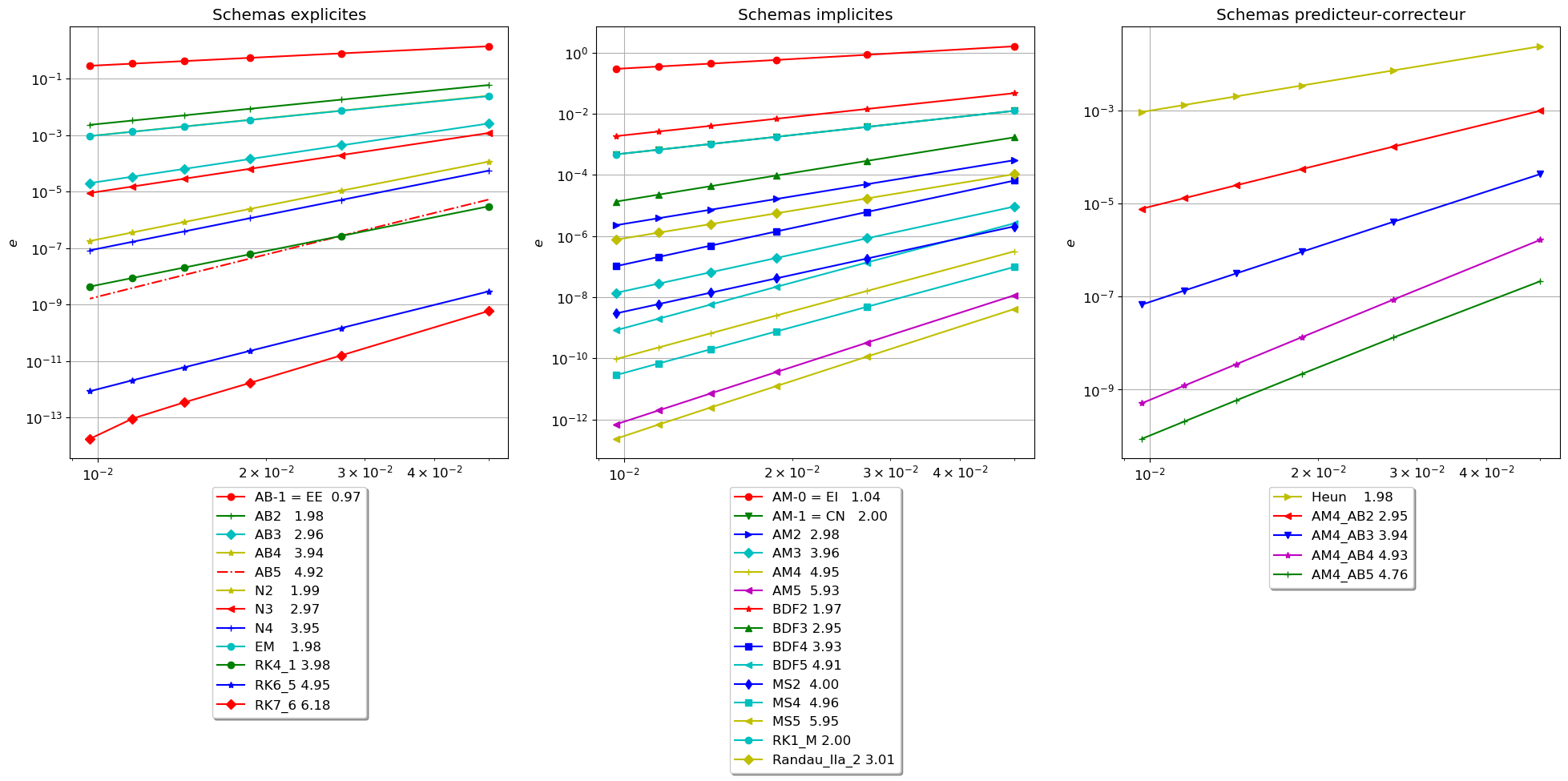
Si on note
alors l’ordre du schéma predictor-corrector est \(\omega_{[PC]}=\min\{\omega_{[C]},\omega_{[P]}+1\}\)
Pour les schémas AM4-ABx, le schéma corrector est d’ordre \(p=5\), pour ne pas perdre en ordre convergence il faut choisir un schéma predictor d’ordre \(p-1\) (ici AB4).
De manière compacte en utilisant une liste des noms des schémas et des dictionnaires:
schemasEXPL = ['EE','AB2','AB3','AB4','AB5','N2','N3','N4', 'EM', 'RK4', 'RK6_5', 'RK7_6']
schemasIMPL = ['EI', 'CN', 'AM2', 'AM3', 'AM4', 'AM5', 'BDF2', 'BDF3', 'BDF4', 'BDF5', 'MS2', 'MS4', 'MS5', 'RK1_M', 'Randau_IIa_2']
schemasPRCO = ['heun', 'AM4AB2', 'AM4AB3', 'AM4AB4', 'AM4AB5']

schemas = schemasEXPL + schemasIMPL + schemasPRCO

H = []
err = { schemas[s] : [] for s in range(len(schemas)) }

N = 10
for k in range(6):
    N += 50
    tt = np.linspace(t0, tfinal, N+1)
    h = tt[1]-tt[0]
    H.append(h)
    yy = np.array([sol_exacte(t) for t in tt])
    uu = { s : eval(s)(phi, tt, sol_exacte) for s in schemas }
    for key in uu:
        err[key].append(np.linalg.norm(uu[key]-yy,np.inf))

ordre = {  key : np.polyfit(np.log(H),np.log(err[key]),1)[0] for key in err  }


plt.figure(figsize=(24,7))
markers=['^', 's', 'p', 'h', '8', 'D', '>', '<', '*','+','o', 'x']

plt.subplot(1,3,1)
for idx,s in enumerate(schemasEXPL):
    plt.loglog(H,err[s], label=f'{s}: {ordre[s]:1.2f}',marker=markers[idx%len(markers)])
plt.xlabel('$h$')
plt.ylabel('$e$')
plt.title("Schemas explicites")
plt.legend(loc='upper center', bbox_to_anchor=(0.5, -0.05), fancybox=True, shadow=True, ncol=1)
plt.grid(True)

plt.subplot(1,3,2)
for idx,s in enumerate(schemasIMPL):
    plt.loglog(H,err[s], label=f'{s}: {ordre[s]:1.2f}',marker=markers[idx%len(markers)])
plt.xlabel('$h$')
plt.ylabel('$e$')
plt.title("Schemas implicites")
plt.legend(loc='upper center', bbox_to_anchor=(0.5, -0.05), fancybox=True, shadow=True, ncol=1)
plt.grid(True)

plt.subplot(1,3,3)
for idx,s in enumerate(schemasPRCO):
    plt.loglog(H,err[s], label=f'{s}: {ordre[s]:1.2f}',marker=markers[idx%len(markers)])
plt.xlabel('$h$')
plt.ylabel('$e$')
plt.title("Schemas predicteur-correcteur")
plt.legend(loc='upper center', bbox_to_anchor=(0.5, -0.05), fancybox=True, ncol=1)
plt.grid(True);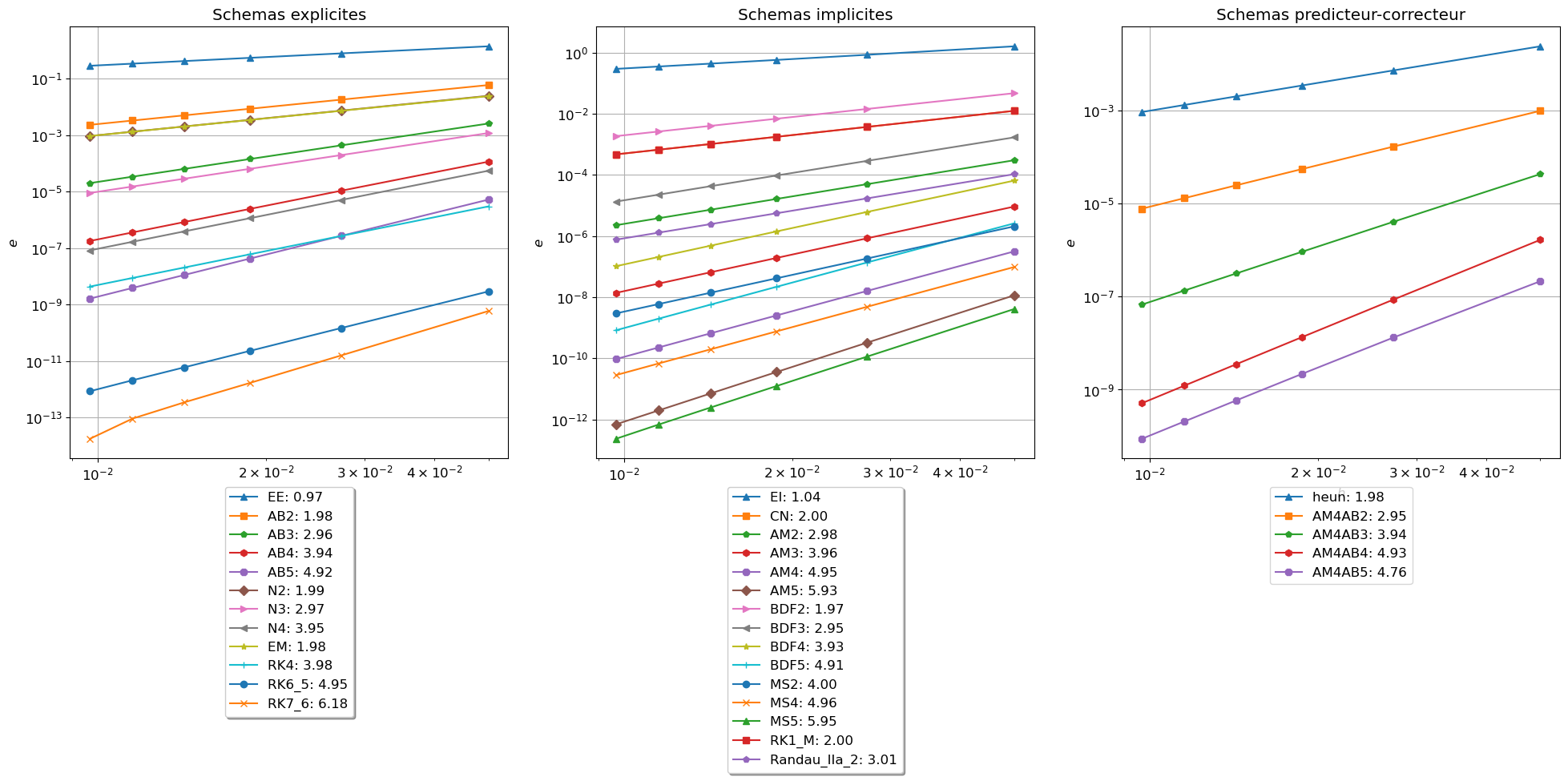
Idem sans utiliser eval :
schemasEXPL = [EE, AB2, AB3, AB4, AB5, N2, N3, N4, EM, RK4, RK6_5, RK7_6]
schemasIMPL = [EI, CN, AM2, AM3, AM4, AM5, BDF2, BDF3, BDF4, BDF5, MS2, MS4, MS5, RK1_M, Randau_IIa_2]
schemasPRCO = [heun, AM4AB2, AM4AB3, AM4AB4, AM4AB5]

schemas = schemasEXPL + schemasIMPL + schemasPRCO

H = []
err = { sfct.__name__ : [] for sfct in schemas }

N = 10
for k in range(6):
    N += 50
    tt = np.linspace(t0, tfinal, N+1)
    h = tt[1]-tt[0]
    H.append(h)
    yy = np.array([sol_exacte(t) for t in tt])
    uu = { sfct.__name__ : sfct(phi, tt, sol_exacte) for sfct in schemas }
    for key in uu:
        err[key].append(np.linalg.norm(uu[key]-yy,np.inf))

ordre = {  key : np.polyfit(np.log(H),np.log(err[key]),1)[0] for key in err  }


plt.figure(figsize=(24,7))
markers=['^', 's', 'p', 'h', '8', 'D', '>', '<', '*','+','o', 'x']

plt.subplot(1,3,1)
for idx,sfct in enumerate(schemasEXPL):
    s = sfct.__name__
    plt.loglog(H,err[s], label=f'{s}: {ordre[s]:1.2f}',marker=markers[idx%len(markers)])
plt.xlabel('$h$')
plt.ylabel('$e$')
plt.title("Schemas explicites")
plt.legend(loc='upper center', bbox_to_anchor=(0.5, -0.05), fancybox=True, shadow=True, ncol=1)
plt.grid(True)

plt.subplot(1,3,2)
for idx,sfct in enumerate(schemasIMPL):
    s = sfct.__name__
    plt.loglog(H,err[s], label=f'{s}: {ordre[s]:1.2f}',marker=markers[idx%len(markers)])
plt.xlabel('$h$')
plt.ylabel('$e$')
plt.title("Schemas implicites")
plt.legend(loc='upper center', bbox_to_anchor=(0.5, -0.05), fancybox=True, shadow=True, ncol=1)
plt.grid(True)

plt.subplot(1,3,3)
for idx,sfct in enumerate(schemasPRCO):
    s = sfct.__name__
    plt.loglog(H,err[s], label=f'{s}: {ordre[s]:1.2f}',marker=markers[idx%len(markers)])
plt.xlabel('$h$')
plt.ylabel('$e$')
plt.title("Schemas predicteur-correcteur")
plt.legend(loc='upper center', bbox_to_anchor=(0.5, -0.05), fancybox=True, ncol=1)
plt.grid(True);