Code
import numpy as np
import matplotlib.pyplot as plt
import sympy as sp
from scipy.optimize import fsolve
from scipy.integrate import solve_ivp, odeint
from IPython.display import display, Markdown, MathDans le sujet il y a plusieurs paramètres. Pour les fixer, remplacez mon nom et prénom par les votres dans les cellules indiquées et vous obtiendrez un choix pour chaque paramètre.
import numpy as np
import matplotlib.pyplot as plt
import sympy as sp
from scipy.optimize import fsolve
from scipy.integrate import solve_ivp, odeint
from IPython.display import display, Markdown, MathOn considère le problème de Cauchy
\( \begin{cases} y'(t)=ay(t)+b(t), & t\in[0;2]\\ y(t_0)=y_0 \end{cases} \)
La méthode d’Euler exponentielle appliquée à ce problème de Cauchy s’écrit comme suit:
\(\text{(EEx) } \begin{cases} u_0=y_0,\\ u_{n+1}=e^{ha}u_n+hg(ha)b(t_n+h/2), & n=0,\dots, N-1 \end{cases} \)
où \(g(z)=\dfrac{e^z-1}{z}\).
La donnée initiale \(y_0\), la constante \(a\), la fonction \(t\mapsto b(t)\) et le nombre de points \(N\) sont donnés dans la cellule ci-dessous (modifiér nom et prénom).
prlat = lambda *args: display(Math(''.join( sp.latex(arg) for arg in args )))


nom = "Faccanoni"
prenom = "Gloria"

print("Paramètres de l'exercice 1")
S = sum([ord(c) for c in nom+prenom])
L = list(range(1,5))
idx = S%len(L)
y0 = L[idx]
prlat("y_0 = ",y0)

L = [ (-10,1), (-10,3), (-10,5), (-5,1), (-5,3) ]
idx = S%len(L)
a,d = L[idx]
c,N = -a, 1-a
prlat("a = ",a)
prlat("b(t) = ",c,"t+",d)
prlat("N = ",N)
Paramètres de l'exercice 1\(\displaystyle \mathtt{\text{y\_0 = }}1\)
\(\displaystyle \mathtt{\text{a = }}-5\)
\(\displaystyle \mathtt{\text{b(t) = }}5\mathtt{\text{t+}}3\)
\(\displaystyle \mathtt{\text{N = }}6\)
Q1 [3 points] Comparer la solution exacte, la solution approchée obtenue par la méthode d’Euler explicite (EE) et la solution obtenue avec la méthode d’Euler exponentielle (EEx) avec \(N+1\) points.
# ======================================================
# variables globales
# ======================================================
t0     = 0
tfinal = 2

# ======================================================
# solution exacte symbolique
# ======================================================
t = sp.Symbol('t')
y = sp.Function('y')

b = lambda t :  c*t+d
phi = lambda t,y :  a*y+b(t)

edo = sp.Eq( sp.diff(y(t),t) , phi(t,y(t)) )
display(edo)
solpar = sp.dsolve(edo, y(t), ics={y(t0):y0})
display(solpar.simplify())

# ======================================================
# solution exacte numérique
# ======================================================
print(f'Choix: {a=}, b(t)={c}t+{d} donc la solution exacte est')

sol_exacte = sp.lambdify(t,solpar.rhs,'numpy')

# ======================================================
# SCHÉMAS
# ======================================================
schemas = ['EEx','EE']
Nb_schemas = len(schemas)

def EEx(phi,tt,y0):
    h = tt[1]-tt[0]
    uu = np.zeros_like(tt)
    uu[0] = y0
    for n in range(len(tt)-1):
        K1 = (np.exp(a*h)-1)/(a*h)
        uu[n+1] = np.exp(a*h)*uu[n]+h*K1*b(tt[n]+h/2)
    return uu

def EE(phi,tt,y0):
    h = tt[1]-tt[0]
    uu = np.zeros_like(tt)
    uu[0] = y0
    for n in range(len(tt)-1):
        uu[n+1] = uu[n]+h*phi(tt[n],uu[n])
    return uu

# ======================================================
# CALCUL SOLUTION APPROCHEE
# ======================================================
tt = np.linspace(t0,tfinal,N+1)
yy = sol_exacte(tt)

uu  = { schemas[s] : eval(schemas[s])(phi,tt,y0) for s in range(Nb_schemas) }
err = { schemas[s] : np.linalg.norm(uu[schemas[s]]-yy,np.inf) for s in range(Nb_schemas) }

plt.figure(figsize=(28,6))
idx = 0
for key in uu:
    plt.subplot(1,Nb_schemas,idx+1)
    plt.plot(tt,yy,'b-',tt,uu[key],'r-D')
    plt.legend(['Exacte', f'{key}, {N=}'])
    plt.title( f'{key} - max(|err|)= {err[key]:g}' )
    idx += 1
\(\displaystyle \frac{d}{d t} y{\left(t \right)} = 5 t - 5 y{\left(t \right)} + 3\)
\(\displaystyle y{\left(t \right)} = t + \frac{2}{5} + \frac{3 e^{- 5 t}}{5}\)
Choix: a=-5, b(t)=5t+3 donc la solution exacte est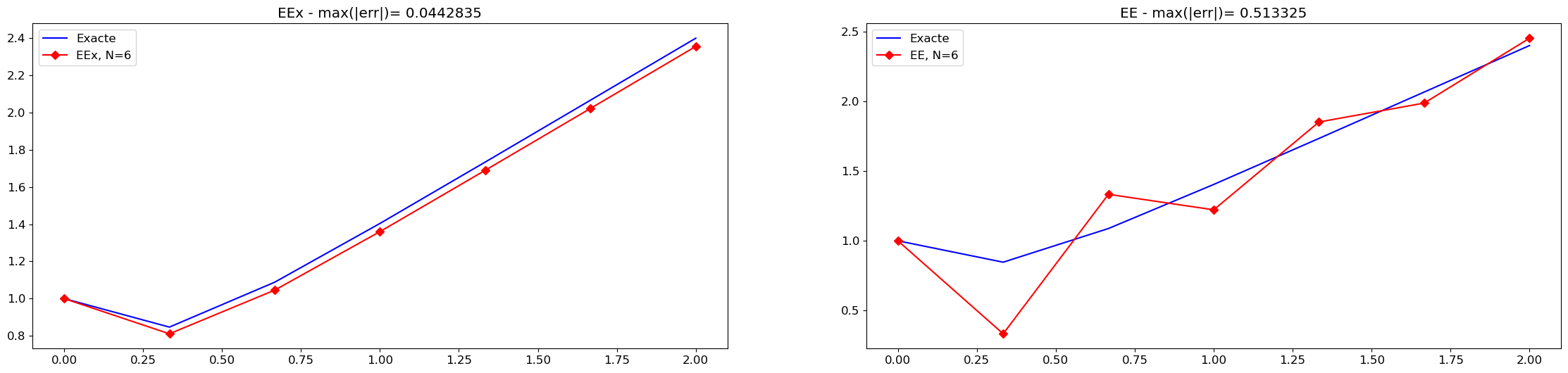
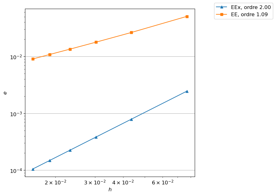
Q2 [2 points] Comparer ensuite empiriquement les ordres de convergence.
# ======================================================
# CALCUL ORDRE
# ======================================================
H = []
err= { schemas[s] : [] for s in range(Nb_schemas) }

plt.figure(figsize=(12,6))
ax = []
for i in range(Nb_schemas):
    ax.append(plt.subplot(1,Nb_schemas,i+1))

for k in range(6):
    N += 20
    h = (tfinal-t0)/N
    H.append(h)
    tt = np.linspace(t0,tfinal,N+1)
    yy = sol_exacte(tt)
    uu = { schemas[s] : eval(schemas[s])(phi,tt,y0) for s in range(Nb_schemas) }
    idx = 0
    for key in uu:
        err[key].append( np.linalg.norm(uu[key]-yy,np.inf) )
        ax[idx].plot(tt,uu[key],label=f'{key}, {N=}')
        idx += 1

for i in range(Nb_schemas):
    ax[i].plot(tt,yy,'b-',label='Exacte')
    ax[i].legend()
    ax[i].set_title(schemas[i])

ordre = {  key : np.polyfit(np.log(H),np.log(err[key]),1)[0] for key in err  }

plt.figure(figsize=(7,7))
markers = ['^', 's', 'p', 'h', '8', 'D', '>', '<', '*','+','o']

for s in range(Nb_schemas):
    plt.loglog(H,err[schemas[s]], label=f'{schemas[s]}, ordre {ordre[schemas[s]]:1.2f}',marker=markers[s])
plt.xlabel('$h$')
plt.ylabel('$e$')
plt.legend(bbox_to_anchor=(1.1, 1.05))
plt.grid(True)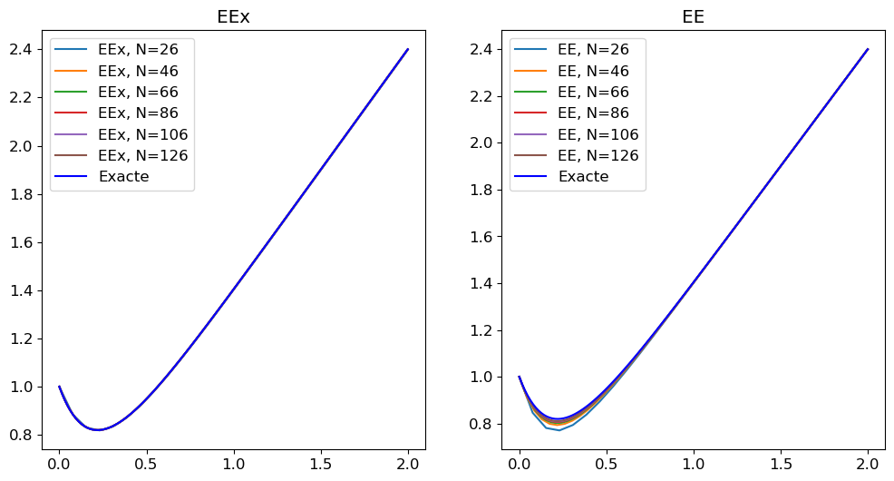
Considérons le schéma dont la matrice de Butcher est donnée ci-dessous:
\( \begin{array}{c|ccc} 0 & 0 & 0 & 0 \\ \dfrac{1}{2} & \dfrac{5}{24} & \dfrac{1}{3}&\dfrac{-1}{24}\\ 1 & 0 &1&0\\ \hline & \dfrac{1}{6} & \dfrac{2}{3} & \dfrac{1}{6} \end{array} \)
Cf. exercice 7.4 page 86 polycopié Christophe Besse
https://www.math.univ-toulouse.fr/~cbesse/mesassets/teaching/L3Mapi3/EDONum/Cours_EDO_C_Besse.pdf
Q1 [1 points] Écrire la suite définie par réccurence associée à ce schéma.
\(\begin{cases} u_0 = y_0 \\ K_1 = \varphi\left(t_n,u_n\right)\\ K_2 = \varphi\left(t_n+\frac{h}{2},u_n+h\left(\frac{5}{24}K_1+\frac{1}{3}K_2-\frac{1}{24}K_3\right)\right)\\ K_3 = \varphi\left(t_{n+1},u_n+hK_2\right)\\ u_{n+1} = u_n + \frac{h}{6}\left(K_1+4K_2+K_3\right) & n=0,1,\dots N-1 \end{cases} \)
Q2 [3 points] Étudier théoriquement l’ordre du schéma.
Soit \(\omega\) l’ordre de la méthode.
C’est un schéma implicite à \(3\) étages (\(s=3\)) donc \(\omega\le2s=6\)
prlat= lambda *args: display(Math(''.join( sp.latex(arg) for arg in args )))

def ordre_RK(s, A=None, b=None, c=None):

    j = sp.symbols('j')

    if A is None:
        A = sp.MatrixSymbol('a', s, s)
    else:
        A = sp.Matrix(A)
    if c is None:
        c = sp.symbols(f'c_0:{s}')
    if b is None:
        b = sp.symbols(f'b_0:{s}')


    display(Markdown("**Matrice de Butcher**"))
    But = matrice_Butcher(s, A, b, c)

    Eqs = []

    # display(Markdown(f"**On a {s+1} conditions pour avoir consistance = pour être d'ordre 1**"))
    # ordre_1(s, A, b, c, j)

    display(Markdown("**On doit ajouter 1 condition pour être d'ordre 2**"))
    Eq_2 = ordre_2(s, A, b, c, j)
    Eqs.append(Eq_2)

    display(Markdown("**On doit ajouter 2 conditions pour être d'ordre 3**"))
    Eq_3 = ordre_3(s, A, b, c, j)
    Eqs.extend(Eq_3)

    display(Markdown("**On doit ajouter 4 conditions pour être d'ordre 4**"))
    Eq_4 = ordre_4(s, A, b, c, j)
    Eqs.extend(Eq_4)

    return Eqs


def matrice_Butcher(s, A, b, c):
    But = sp.Matrix(A)
    But = But.col_insert(0, sp.Matrix(c))
    last = [sp.Symbol(" ")]
    last.extend(b)
    But = But.row_insert(s,sp.Matrix(last).T)
    display(Math(sp.latex(sp.Matrix(But))))
    return But


def ordre_1(s, A, b, c, j):
    texte = r"\sum_{j=1}^s b_j =" + f"{sum(b).simplify()}"
    texte += r"\text{ doit être égale à }1"
    display(Math(texte))
    for i in range(s):
        somma = sp.summation(A[i,j],(j,0,s-1)).simplify()
        texte = r'\sum_{j=1}^s a_{'+str(i)+r'j}=' + sp.latex( somma )
        texte += r"\text{ doit être égale à }"+sp.latex(c[i])
        display(Math( texte ))
    return None


def ordre_2(s, A, b, c, j):
    texte = r'\sum_{j=1}^s b_j c_j=' +sp.latex(sum([b[i]*c[i] for i in range(s)]).simplify())
    texte += r"\text{ doit être égale à }\frac{1}{2}"
    display(Math(texte))
    Eq_2 = sp.Eq( sum([b[i]*c[i] for i in range(s)]).simplify(), sp.Rational(1,2) )
    return Eq_2


def ordre_3(s, A, b, c, j):
    texte = r'\sum_{j=1}^s b_j c_j^2='
    texte += sp.latex( sum([b[i]*c[i]**2 for i in range(s)]).simplify() )
    texte += r"\text{ doit être égale à }\frac{1}{3}"
    display(Math(texte))
    Eq_3_1 = sp.Eq( sum([b[i]*c[i]**2 for i in range(s)]).simplify(), sp.Rational(1,3) )
    texte = r'\sum_{i,j=1}^s b_i a_{ij} c_j='
    somma = sum([b[i]*A[i,j]*c[j] for j in range(s) for i in range(s)]).simplify()
    texte = texte + sp.latex(somma)
    texte += r"\text{ doit être égale à }\frac{1}{6}"
    display(Math(texte))
    Eq_3_2 = sp.Eq( sum([b[i]*A[i,j]*c[j] for j in range(s) for i in range(s)]).simplify(), sp.Rational(1,6) )
    return [Eq_3_1, Eq_3_2]


def ordre_4(s, A, b, c, j):
    texte = r'\sum_{j=1}^s b_j c_j^3='
    texte += sp.latex( sum([b[i]*c[i]**3 for i in range(s)]).simplify() )
    texte += r"\text{ doit être égale à }\frac{1}{4}"
    display(Math(texte))
    Eq_4_1 = sp.Eq( sum([b[i]*c[i]**3 for i in range(s)]).simplify(), sp.Rational(1,4) )
    texte = r'\sum_{i,j=1}^s b_i c_i a_{ij} c_j='
    somma = sum([b[i]*c[i]*A[i,j]*c[j] for j in range(s) for i in range(s)]).simplify()
    texte = texte + sp.latex(somma)
    texte += r"\text{ doit être égale à }\frac{1}{8}"
    display(Math(texte))
    Eq_4_2 = sp.Eq( sum([b[i]*c[i]*A[i,j]*c[j] for j in range(s) for i in range(s)]).simplify(), sp.Rational(1,8) )
    texte = r'\sum_{i,j=1}^s b_i a_{ij} c_j^2='
    somma = sum([b[i]*A[i,j]*c[j]**2 for j in range(s) for i in range(s)]).simplify()
    texte = texte + sp.latex(somma)
    texte += r"\text{ doit être égale à }\frac{1}{12}"
    display(Math(texte))
    Eq_4_3 = sp.Eq( sum([b[i]*A[i,j]*c[j]**2 for j in range(s) for i in range(s)]).simplify(), sp.Rational(1,12) )
    texte = r'\sum_{i,j,k=1}^s b_i a_{ij} a_{jk} c_k='
    somma = sum([b[i]*A[i,j]*A[j,k]*c[k] for k in range(s) for j in range(s) for i in range(s)]).simplify()
    texte = texte + sp.latex(somma)
    texte += r"\text{ doit être égale à }\frac{1}{24}"
    display(Math(texte))
    Eq_4_4 = sp.Eq( sum([b[i]*A[i,j]*A[j,k]*c[k] for k in range(s) for j in range(s) for i in range(s)]).simplify(), sp.Rational(1,24) )
    return [Eq_4_1, Eq_4_2, Eq_4_3, Eq_4_4]


##################################################
# Conditions avec s étages
##################################################

c = [0,sp.Rational(1,2),1]
b = [sp.Rational(1,6),sp.Rational(2,3),sp.Rational(1,6)]
A = [ [0,0,0],
      [sp.Rational(5,24),sp.Rational(1,3),-sp.Rational(1,24)],
      [0,1,0]]
s = len(c)

Eqs = ordre_RK(s, A, b, c)

# for eq in Eqs:
#     display(eq)
#
Matrice de Butcher
\(\displaystyle \left[\begin{matrix}0 & 0 & 0 & 0\\\frac{1}{2} & \frac{5}{24} & \frac{1}{3} & - \frac{1}{24}\\1 & 0 & 1 & 0\\ & \frac{1}{6} & \frac{2}{3} & \frac{1}{6}\end{matrix}\right]\)
On doit ajouter 1 condition pour être d’ordre 2
\(\displaystyle \sum_{j=1}^s b_j c_j=\frac{1}{2}\text{ doit être égale à }\frac{1}{2}\)
On doit ajouter 2 conditions pour être d’ordre 3
\(\displaystyle \sum_{j=1}^s b_j c_j^2=\frac{1}{3}\text{ doit être égale à }\frac{1}{3}\)
\(\displaystyle \sum_{i,j=1}^s b_i a_{ij} c_j=\frac{1}{6}\text{ doit être égale à }\frac{1}{6}\)
On doit ajouter 4 conditions pour être d’ordre 4
\(\displaystyle \sum_{j=1}^s b_j c_j^3=\frac{1}{4}\text{ doit être égale à }\frac{1}{4}\)
\(\displaystyle \sum_{i,j=1}^s b_i c_i a_{ij} c_j=\frac{1}{8}\text{ doit être égale à }\frac{1}{8}\)
\(\displaystyle \sum_{i,j=1}^s b_i a_{ij} c_j^2=\frac{5}{72}\text{ doit être égale à }\frac{1}{12}\)
\(\displaystyle \sum_{i,j,k=1}^s b_i a_{ij} a_{jk} c_k=\frac{5}{144}\text{ doit être égale à }\frac{1}{24}\)
D’après ces résultats, le schéma est d’ordre \(3\).
Q3 [4 points] Étudier théoriquement la A-stabilité du schéma.
La méthode appliquée à l’EDO \(y'(t)=-\beta y(t)\) avec \(\beta>0\) s’écrit: \(\begin{cases} u_0 = y_0 \\ K_1 = -\beta u_n\\ K_2 = -\beta\left(u_n+\frac{h}{24}\left(5K_1+8K_2-K_3\right)\right)\\ K_3 = -\beta\left(u_n+hK_2\right)\\ u_{n+1} = u_n + \frac{h}{6}\left(K_1+4K_2+K_3\right) & n=0,1,\dots N-1 \end{cases} \)
En effet, si on note \(x=\beta h\), par induction on obtient \( u_{n}=\left(-\frac{x^3-5x^2+16x-24}{x^2+8x+24}\right)^nu_0. \) Par conséquent, \(\lim\limits_{n\to+\infty}u_n=0\) si et seulement si \( \left|\frac{x^3-5x^2+16x-24}{x^2+8x+24}\right|<1. \)
L’étude de la fonction \(x\mapsto\frac{x^3-5x^2+16x-24}{x^2+8x+24}\) pour \(x>0\) montre que le schéma est A-stable ssi \(h<\frac{6}{\beta}\).
u_n, h, beta, K1, K2, K3 = sp.symbols(r'u_n h \beta K_1 K_2 K_3')

g = lambda y : -beta*y

eq1 = sp.Eq( K1 , g(u_n))
eq2 = sp.Eq( K2 , g(u_n+h*5/24*K1+h/3*K2-h/24*K3) )
eq3 = sp.Eq( K3 , g(u_n+h*K2) )
sol = sp.solve([eq1,eq2,eq3],[K1,K2,K3])
for key in sol:
    texte = sp.latex(key) + "=" + sp.latex(sol[key])
    display(Math(texte))

RHS = u_n+h/6*(K1+2*K2+K3)
RHS = RHS.subs(sol).simplify()
texte = 'u_{n+1}=' + sp.latex(RHS)
display(Math(texte))

display(Markdown(r"Notons $x=h\beta>0$. On trouve donc"))
x = sp.Symbol('x',positive=True)
RHS = RHS.subs(h*beta,x).simplify()
texte = 'u_{n+1}=' + sp.latex(RHS)
display(Math(texte))
texte = r"\text{La méthode est A-stable ssi }|q(x)|<1\text{ avec }q(x)=\frac{u_{n+1}}{u_n}="
texte += sp.latex(RHS/u_n)
display(Math(texte))
sp.solve([-1<RHS/u_n,RHS/u_n<1])
\(\displaystyle K_{1}=- \beta u_{n}\)
\(\displaystyle K_{2}=\frac{4 \beta^{2} h u_{n} - 24 \beta u_{n}}{\beta^{2} h^{2} + 8 \beta h + 24}\)
\(\displaystyle K_{3}=\frac{- 5 \beta^{3} h^{2} u_{n} + 16 \beta^{2} h u_{n} - 24 \beta u_{n}}{\beta^{2} h^{2} + 8 \beta h + 24}\)
\(\displaystyle u_{n+1}=\frac{u_{n} \left(- 3 \beta^{3} h^{3} + 11 \beta^{2} h^{2} - 24 \beta h + 72\right)}{3 \left(\beta^{2} h^{2} + 8 \beta h + 24\right)}\)
Notons \(x=h\beta>0\). On trouve donc
\(\displaystyle u_{n+1}=\frac{u_{n} \left(- 3 x^{3} + 11 x^{2} - 24 x + 72\right)}{3 \left(x^{2} + 8 x + 24\right)}\)
\(\displaystyle \text{La méthode est A-stable ssi }|q(x)|<1\text{ avec }q(x)=\frac{u_{n+1}}{u_n}=\frac{- 3 x^{3} + 11 x^{2} - 24 x + 72}{3 \left(x^{2} + 8 x + 24\right)}\)
\(\displaystyle x < 6\)
q = -RHS/u_n
display( Math (r'-\frac{u_{n+1}}{u_n}=' + sp.latex(q) + "=:q(x)") )
display( Math (r'q(0)=' + sp.latex(q.subs(x,0)) ) )
display( Math (r'\lim_{x\to+\infty}q(x)=' + sp.latex(q.limit(x,sp.oo)) ) )
dq = sp.diff(q,x).simplify()
display( Math ( r"q'(x)=" + sp.latex(dq) ) )
display( Math ( r"q'(x)>0 \text{ ? } " + sp.latex(sp.solve(dq>0)) ) )
display( Math ( r"q(x)=1 \iff x= " + sp.latex(sp.solve(q-1)) ) )
# prlat( r"q(x)=0 \iff x= " ,[ xi.evalf() for xi in sp.solve(q)] )

xx = np.linspace(0,8,100)
yy = (xx**3-5*xx**2+16*xx-24)/(xx**2+8*xx+24)
plt.plot(xx,yy)
plt.plot([xx[0],xx[-1]],[-1,-1])
plt.plot([xx[0],xx[-1]],[1,1])
plt.grid();
\(\displaystyle -\frac{u_{n+1}}{u_n}=- \frac{- 3 x^{3} + 11 x^{2} - 24 x + 72}{3 \left(x^{2} + 8 x + 24\right)}=:q(x)\)
\(\displaystyle q(0)=-1\)
\(\displaystyle \lim_{x\to+\infty}q(x)=\infty\)
\(\displaystyle q'(x)=\frac{x^{4} + 16 x^{3} + \frac{104 x^{2}}{3} - 128 x + 384}{x^{4} + 16 x^{3} + 112 x^{2} + 384 x + 576}\)
\(\displaystyle q'(x)>0 \text{ ? } \text{True}\)
\(\displaystyle q(x)=1 \iff x= \left[ 6\right]\)
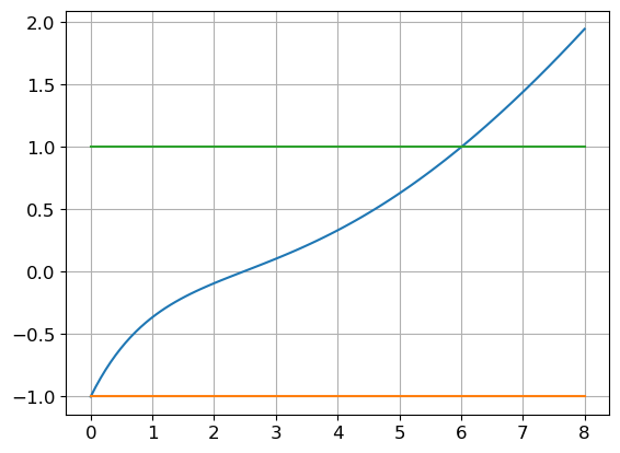
Elle est strictement croissante sur \([0,+\infty[\), \(q(0)=-1\) et \(\lim\limits_{x\to+\infty}q(x)=+\infty\). Il existe donc un et un seul \(x_0\) tel que \(q(x_0)=1\). En résolvant l’équation on trouve \(x_0=6\).
La condition de stabilité est donc satisfaite ssi \(0<x<6\), donc ssi \( h<\frac{6}{\beta}. \)
Q4 [3 points] Considérons le problème de Cauchy \(y'(t)=-50y(t)\) pour \(t\in]0,1]\) et \(y(0)=1\).
Vérifier empiriquement qu’avec \(N=8\) (i.e. 9 points de discrétisation) le schéma est instable et avec \(N=21\) il est stable.
# variables globales
t0     = 0
tfinal = 1
y0     = 1
beta      = 50

phi = lambda t,y: -beta*y

##############################################
# solution exacte
##############################################
sol_exacte = lambda t : y0*np.exp(-beta*t)

##############################################
# solution approchée
##############################################
def RK(tt,phi,y0):
    h = tt[1]-tt[0]
    uu = np.zeros_like(tt)
    uu[0] = y0
    for n in range(len(tt)-1):
        K1 = phi(tt[n],uu[n])
        sys = lambda X : [-X[0]+phi(tt[n]+h/2,uu[n]+h*(5/24*K1+X[0]/3-X[1]/24)) ,
                          -X[1]+phi(tt[n+1],uu[n]+h*X[0])]
        K2, K3 = fsolve( sys , [K1,K1] )
        uu[n+1] = uu[n]+h/6*(K1+4*K2+K3)
    return uu

##############################################
# ordre
##############################################
# 6/beta>h=(tfinal-t0)/N
# N>(tfinal-t0)*beta/6

plt.figure(figsize=(16,5))

plt.subplot(1,2,1)
N = int((tfinal-t0)*beta/6)
tt = np.linspace(t0, tfinal, N + 1)
h  = tt[1] - tt[0]
yy = sol_exacte(tt)
uu = RK(tt, phi, y0)
err = np.linalg.norm(uu-yy,np.inf)
plt.plot(tt,uu,label=f'Approchée avec N={N}')
plt.plot(tt,yy,label='Exacte')
plt.xlabel('$t$')
plt.ylabel('$y$')
plt.grid(True)
plt.legend();

plt.subplot(1,2,2)
N = int(int((tfinal-t0)*beta/6)*2.46115761806205+2)
tt = np.linspace(t0, tfinal, N + 1)
h  = tt[1] - tt[0]
yy = sol_exacte(tt)
uu = RK(tt, phi, y0)
err = np.linalg.norm(uu-yy,np.inf)
plt.plot(tt,uu,label=f'Approchée avec N={N}')
plt.plot(tt,yy,label='Exacte')
plt.xlabel('$t$')
plt.ylabel('$y$')
plt.grid(True)
plt.legend();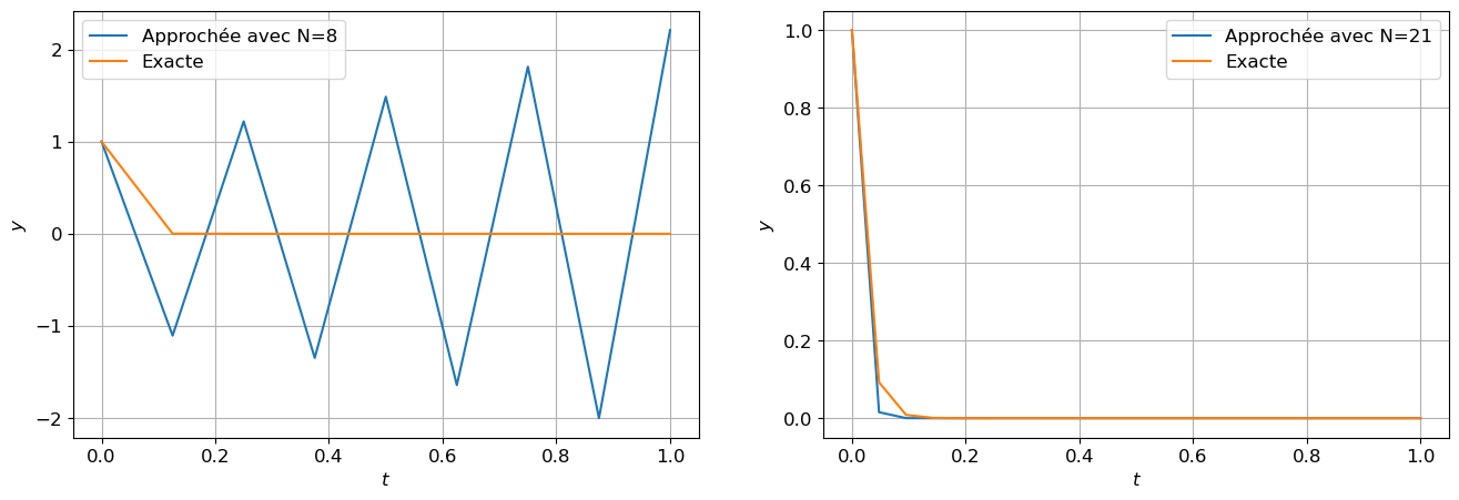
Annexe: calculons la suite géométrique pour étudier la A-stabilité dans le cas générale d’un schéma dont la matrice de Butcher est
\( \begin{array}{c|ccc} 0 & 0 & 0 & 0 \\ c_2 & a_{21} & a_{22}&a_{23}\\ 1 & 0 &1&0\\ \hline & b_1 & b_2 & b_3 \end{array} \)
u_n, h, beta, K1, K2, K3 = sp.symbols(r'u_n h \beta K_1 K_2 K_3')
b_1, b_2, b_3, a_21, a_22, a_23 = sp.symbols(r'b_1 b_2 b_3 a_{21} a_{22} a_{23}')
g = lambda y : -beta*y
eq1 = sp.Eq( K1 , g(u_n))
eq2 = sp.Eq( K2 , g(u_n+h*a_21*K1+h*a_22*K2+h*a_23*K3) )
eq3 = sp.Eq( K3 , g(u_n+h*K2) )
sol = sp.solve([eq1,eq2,eq3],[K1,K2,K3])
for key in sol:
    texte = sp.latex(key) + "=" + sp.latex(sol[key])
    display(Math(texte))
RHS = u_n+h*(b_1*K1+b_2*K2+b_3*K3)
RHS = RHS.subs(sol).simplify()
display(Math( 'u_{n+1}=' + sp.latex(RHS) ))
RHS = RHS.subs(h,x/beta).simplify()
display(Math( 'u_{n+1}=' + sp.latex(RHS) ))
print("Avec nos paramètres on obtient bien:")
RHS = RHS.subs({a_21:5/sp.S(24),a_22:1/sp.S(3),a_23:-1/sp.S(24),b_1:1/sp.S(6),b_2:4/sp.S(6),b_3:1/sp.S(6)}).simplify()
display(Math( 'u_{n+1}=' + sp.latex(RHS) ))
\(\displaystyle K_{1}=- \beta u_{n}\)
\(\displaystyle K_{2}=\frac{- \beta^{2} a_{21} h u_{n} - \beta^{2} a_{23} h u_{n} + \beta u_{n}}{\beta^{2} a_{23} h^{2} - \beta a_{22} h - 1}\)
\(\displaystyle K_{3}=\frac{\beta^{3} a_{21} h^{2} u_{n} + \beta^{2} a_{22} h u_{n} - \beta^{2} h u_{n} + \beta u_{n}}{\beta^{2} a_{23} h^{2} - \beta a_{22} h - 1}\)
\(\displaystyle u_{n+1}=\frac{u_{n} \left(- \beta^{2} a_{23} h^{2} + \beta a_{22} h - \beta h \left(b_{1} \left(- \beta^{2} a_{23} h^{2} + \beta a_{22} h + 1\right) - b_{2} \left(\beta a_{21} h + \beta a_{23} h - 1\right) + b_{3} \left(\beta^{2} a_{21} h^{2} + \beta a_{22} h - \beta h + 1\right)\right) + 1\right)}{- \beta^{2} a_{23} h^{2} + \beta a_{22} h + 1}\)
\(\displaystyle u_{n+1}=\frac{u_{n} \left(a_{22} x - a_{23} x^{2} - x \left(b_{1} \left(a_{22} x - a_{23} x^{2} + 1\right) - b_{2} \left(a_{21} x + a_{23} x - 1\right) + b_{3} \left(a_{21} x^{2} + a_{22} x - x + 1\right)\right) + 1\right)}{a_{22} x - a_{23} x^{2} + 1}\)
Avec nos paramètres on obtient bien:\(\displaystyle u_{n+1}=\frac{u_{n} \left(- x^{3} + 5 x^{2} - 16 x + 24\right)}{x^{2} + 8 x + 24}\)
On s’intèresse au problème de Cauchy
\( \begin{cases} y'(t)=\varphi_1(t,y(t),z(t)),\\ z'(t)=\varphi_2(t,y(t),z(t)),\\ y(0)=y_0,\\ z(0)=z_0 \end{cases} \)
Soit \(H\colon (y,z)\mapsto H(y,z)\) une fonction de deux variables régulière et posons \(\varphi_1(t,y,z)=\dfrac{\partial H}{\partial z}\) et \(\varphi_2(t,y,z)=-\dfrac{\partial H}{\partial y}\).
Notons \(\mathcal{H}\colon t \mapsto H(y(t),z(t))\). Montrer que \(\mathcal{H}\) est constante.
Posons \(H(y,z)=\dfrac{(ay)^2+(bz)^2}{2}\) où \(a\) et \(b\) sont des constantes fixées dans la cellule précédente.
Dans la suite on notera \(u_n\approx y(t_n)\), \(w_n\approx z(t_n)\) et \(J_n\approx\mathcal{H}(t_n)\). Calculer la solution approchée obtenue par la méthode suivante appelée méthode d’Euler symplectique.
\( \text{(ES) }\begin{cases}
u_0=y_0,\\
w_0=z_0,\\
u_{n+1}=u_n+h\varphi_1\left(t_n,u_n,w_n\right),\\
w_{n+1}=w_n+h\varphi_2\left(t_{n+1},u_{n+1},w_{n+1}\right).
\end{cases} \)
Nota bene: le choix particulier de \(\varphi_1\) et \(\varphi_2\) permet de réécrire le schéma sous forme explicite.
Dans trois répère différents afficher, en comparant solution exacte et solution approchée,
Q1 [1 point] Notons \(\mathcal{H}\colon t \mapsto H(y(t),z(t))\). Montrer que \(\mathcal{H}\) est constante.
On a \( \mathcal{H}'(t)= \frac{d }{dt}H(y(t),z(t))= \frac{\partial H}{\partial y}y'(t)+\frac{\partial H}{\partial z}z'(t)= -z'(t)y'(t)+y'(t)z'(t)=0. \)
prlat= lambda *args: display(Math(''.join( sp.latex(arg) for arg in args )))

nom = "Faccanoni"
prenom = "Gloria"

print("Paramètres de l'exercice 3")
L = [ (-1,0),(1,0),(0,1),(0,-1) ]
idx = sum([ord(c) for c in nom+prenom])%len(L)
y0,z0 = L[idx]
prlat("y_0 = ",y0)
prlat("z_0 = ",z0)

L = [ (1,2),(2,1),(3,2),(2,3),(3,1),(1,3) ]
idx = sum([ord(c) for c in nom+prenom])%len(L)
(a,b) = L[idx]
prlat("a = ",a)
prlat("b = ",b)
Paramètres de l'exercice 3\(\displaystyle \mathtt{\text{y\_0 = }}-1\)
\(\displaystyle \mathtt{\text{z\_0 = }}0\)
\(\displaystyle \mathtt{\text{a = }}3\)
\(\displaystyle \mathtt{\text{b = }}1\)
Q2 [2 point] Posons \(H(y,z)=\dfrac{(ay)^2+(bz)^2}{2}\) où \(a\) et \(b\) sont des constantes fixées dans la cellule précédente.
Calculer la solution exacte (les données initiales sont fixées dans la cellule précédente).
Dans la suite on posera \(T=4\pi/(ab)\) et, pour les affichages, on chosira \(N+1\) points avec \(N=48\).
Dans trois répères différents afficher
- \(t\mapsto y(t)\) et \(t\mapsto z(t)\) dans le même répère,
- \(y\mapsto z(y)\),
- \(t\mapsto\mathcal{H}(t)\).
Le problème de Cauchy devient
\( \begin{cases} y'(t)=b^2z(t),\\ z'(t)=-a^2y(t),\\ y(0)=y_0,\\ z(0)=z_0 \end{cases} \)
t0 = 0

tfinal = 4*np.pi/(a*b)
N = 48

phi1 = lambda t,y,z : b**2*z
phi2 = lambda t,y,z : -a**2*y
Ham = lambda y,z : ((a*y)**2+(b*z)**2)/2
La solution exacte est
_h = sp.Symbol('h',positive=True)

_phi1 = lambda t,y,z :  sp.diff(Ham(y,z),z)
_phi2 = lambda t,y,z : -sp.diff(Ham(y,z),y)

t = sp.Symbol('t')
y = sp.Function('y')
z = sp.Function('z')

edo1 = sp.Eq( sp.diff(y(t),t) , _phi1(t,y(t),z(t)) )
edo2 = sp.Eq( sp.diff(z(t),t) , _phi2(t,y(t),z(t)) )
# display(edo1)
# display(edo2)
solpar_1, solpar_2 = sp.dsolve([edo1,edo2],[y(t),z(t)], ics={y(t0):y0, z(t0):z0})

display(solpar_1,solpar_2)
\(\displaystyle y{\left(t \right)} = - \cos{\left(3 t \right)}\)
\(\displaystyle z{\left(t \right)} = 3 \sin{\left(3 t \right)}\)
Les trois graphes sont
func_1 = sp.lambdify(t,solpar_1.rhs,'numpy')
func_2 = sp.lambdify(t,solpar_2.rhs,'numpy')

tt = np.linspace(t0,tfinal,N+1)
h  = tt[1]-tt[0]

plt.figure(figsize=(18,5))
yy = func_1(tt)
zz = func_2(tt)
HH = [ Ham(y,z) for (y,z) in zip(yy,zz) ]

plt.subplot(1,3,1)
plt.plot(tt,yy,'-*',tt,zz,'-*')
plt.legend([r'$t\mapsto y(t)$',r'$t\mapsto z(t)$'])
plt.xlabel(r'$t$')

plt.subplot(1,3,2)
plt.plot(yy,zz,'-*')
plt.xlabel(r'$y$')
plt.ylabel(r'$z$')
plt.axis('equal')

plt.subplot(1,3,3)
plt.plot(tt,HH,'-*')
plt.xlabel(r'$t$')
plt.ylabel(r'$\mathcal{H}$')
plt.axis('equal');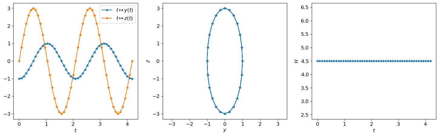
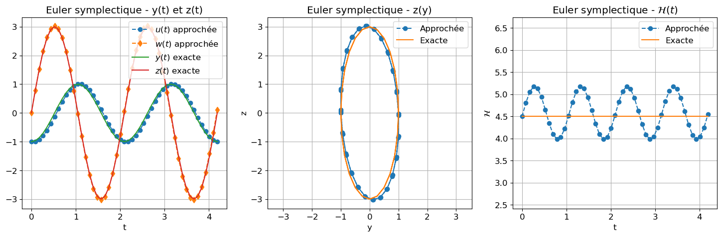
Q3 [4 points]
Dans la suite on notera \(u_n\approx y(t_n)\), \(w_n\approx z(t_n)\) et \(J_n\approx\mathcal{H}(t_n)\).Calculer la solution approchée obtenue par la méthode suivante appelée méthode d’Euler symplectique.
\(\text{(ES) }\begin{cases} u_0=y_0,\\ w_0=z_0,\\ u_{n+1}=u_n+h\varphi_1\left(t_n,u_n,w_n\right),\\ w_{n+1}=w_n+h\varphi_2\left(t_{n+1},u_{n+1},w_{n+1}\right). \end{cases}\)
Nota bene: le choix particulier de \(\varphi_1\) et \(\varphi_2\) permet de réécrire le schéma sous forme explicite.
Dans trois répère différents afficher, en comparant solution exacte et solution approchée,
- \(\{(t_i,u_i)\}\) et \(\{(t_i,w_i)\}\) dans un même répère,
- \(\{(u_i,w_i)\}\),
- \(\{(t_i,J_i)\}\) où \(J_i=H(u_i,w_i)\).
Pour l’affichage des solutions exactes VS approchées, on peut écrire une fonction qui prend en paramètres la discrétisation tt, les deux listes solution exacte yy et zz, les deux listes solution approchée uu et ww, puis une chaîne de caractères s qui contient le nom du schéma, et pour finir HH la liste qui contient le calcul de l’Hamiltonien exact et HH_num celui approché.
def affichage(tt,yy,zz,uu,ww,s,HH,HH_num):

    plt.subplot(1,3,1)
    plt.plot(tt,uu,'o--',tt,ww,'d--')
    plt.plot(tt,yy,tt,zz)
    plt.xlabel('t')
    plt.legend([r'$u(t)$ approchée',r'$w(t)$ approchée','$y(t)$ exacte','$z(t)$ exacte'])
    plt.title(f'{s} - y(t) et z(t)')
    plt.grid()

    plt.subplot(1,3,2)
    plt.plot(uu,ww,'o--')
    plt.plot(yy,zz)
    plt.xlabel('y')
    plt.ylabel('z')
    plt.legend(['Approchée','Exacte'])
    plt.title(f'{s} - z(y)')
    plt.grid()
    plt.axis('equal')

    plt.subplot(1,3,3)
    plt.plot(tt,HH_num,'o--')
    plt.plot(tt,HH)
    plt.xlabel('t')
    plt.ylabel(r'$\mathcal{H}$')
    plt.legend(['Approchée','Exacte'])
    plt.title(f'{s} - '+r'$\mathcal{H}(t)$')
    plt.grid()
    plt.axis('equal');
Le schéma se réécrit
\(\text{(ES) }\begin{cases} u_0=y_0,\\ w_0=z_0,\\ u_{n+1}=u_n+h b^2 w_n,\\ w_{n+1}=-a^2h u_n + (1-(abh)^2)w_n. \end{cases}\)
et
\( J_{n+1}= \frac{(au_{n+1})^2+(bw_{n+1})^2}{2} \)
Vérifions nos calculs:
_h = sp.Symbol('h')
t_n = sp.Symbol('t_n')
u_n = sp.Symbol('u_n')
w_n = sp.Symbol('w_n')
t_np1 = t_n+h
u_np1 = sp.Symbol('u_{n+1}')
w_np1 = sp.Symbol('w_{n+1}')
eq1 = sp.Eq( u_np1 , u_n+_h*_phi1(t_n,u_n,w_n))
eq2 = sp.Eq( w_np1 , w_n+_h*_phi2(t_np1,u_np1,w_np1))
sol = sp.solve([eq1,eq2],[u_np1,w_np1])
prlat( 'u_{n+1}=' , sol[u_np1] )
prlat( 'w_{n+1}=' , sol[w_np1].factor(w_n) )
# prlat( 'H_{n+1}=' , _Ham(sol[u_np1],sol[w_np1]).expand().simplify() )
\(\displaystyle \mathtt{\text{u\_\{n+1\}=}}h w_{n} + u_{n}\)
\(\displaystyle \mathtt{\text{w\_\{n+1\}=}}- 9 h u_{n} - w_{n} \left(9 h^{2} - 1\right)\)
# x0, y0, h variables globales
def ES(phi1,phi2,tt):
    h = tt[1]-tt[0]
    uu = np.zeros_like(tt)
    ww = np.zeros_like(tt)
    uu[0] = y0
    ww[0] = z0
    for n in range(len(tt)-1):
        # uu[n+1] = uu[n]+h*phi1(tt[n],uu[n],ww[n])
        # ww[n+1] = ww[n]+h*phi2(tt[n+1],uu[n+1],None)
        # idem que
        uu[n+1] = uu[n]+h*b**2*ww[n]
        ww[n+1] = -a**2*h*uu[n]+(1-(a*b*h)**2)*ww[n]
    return [uu,ww]

[uu, ww] = ES(phi1,phi2,tt)
HH_num = Ham(uu,ww)

plt.figure(figsize=(18,5))
affichage(tt,yy,zz,uu,ww,"Euler symplectique",HH,HH_num)