Netflix User Data
L’ensemble de données fu fichier Netflix_Userbase.csv fournit un aperçu d’un échantillon d’utilisateurs de Netflix.
Chaque ligne représente un utilisateur unique, identifié par son ID utilisateur.
L’ensemble de données comprend les colonnes suivantes :
- le type d’abonnement de l’utilisateur (Basic, Standard ou Premium),
- le revenu mensuel généré par son abonnement,
- la date d’inscription à Netflix,
- la date de son dernier paiement et
- le pays dans lequel il se trouve.
Des colonnes supplémentaires ont été incluses pour fournir des informations sur le comportement et les préférences des utilisateurs, comme le type d’appareil.
Source : Kaggle
Disclaimer: l’ensemble de données sert de représentation synthétique et ne reflète pas les données réelles des utilisateurs de Netflix.
1 Exercice
- Affichages
- Charger le fichier
Netflix_Userbase.csvdans un DataFrame. - Afficher les 20 premières lignes.
- Combien de ligne et de colonnes contient ce fichier ?
- Quels sont les types des colonnes ?
- Pour chaque colonnes, combien de valeurs différentes contient-elle ?
- Y a-t-il des valeurs manquantes ?
- Charger le fichier
- Modification des données
- Ne garder que les utilisateurs europeens.
- Aggregations/Visualisations
- Afficher le nombre d’utilisateurs par pays.
- Afficher le nombre d’utilisateurs par sexe.
- Afficher le nombre d’utilisateurs par devices utilisés.
- Continuer l’analyse des données en affichant des visualisations qui vous semblent pertinentes en combinant les différentes caractéristiques des utilisateurs.
- Conclusion
- Quels sont les insights que vous avez pu tirer de cette analyse ?
1.1 Affichages
# Importer le jeu de données
df_complet = pd.read_csv('Netflix_Userbase.csv', sep=',', low_memory=False)

# Afficher les 20 premières lignes
df_complet.head(20)| User ID | Subscription Type | Monthly Revenue | Join Date | Last Payment Date | Country | Age | Gender | Device | Plan Duration | |
|---|---|---|---|---|---|---|---|---|---|---|
| 0 | 1 | Basic | 10 | 15-01-22 | 10-06-23 | United States | 28 | Male | Smartphone | 1 Month |
| 1 | 2 | Premium | 15 | 05-09-21 | 22-06-23 | Canada | 35 | Female | Tablet | 1 Month |
| 2 | 3 | Standard | 12 | 28-02-23 | 27-06-23 | United Kingdom | 42 | Male | Smart TV | 1 Month |
| 3 | 4 | Standard | 12 | 10-07-22 | 26-06-23 | Australia | 51 | Female | Laptop | 1 Month |
| 4 | 5 | Basic | 10 | 01-05-23 | 28-06-23 | Germany | 33 | Male | Smartphone | 1 Month |
| 5 | 6 | Premium | 15 | 18-03-22 | 27-06-23 | France | 29 | Female | Smart TV | 1 Month |
| 6 | 7 | Standard | 12 | 09-12-21 | 25-06-23 | Brazil | 46 | Male | Tablet | 1 Month |
| 7 | 8 | Basic | 10 | 02-04-23 | 24-06-23 | Mexico | 39 | Female | Laptop | 1 Month |
| 8 | 9 | Standard | 12 | 20-10-22 | 23-06-23 | Spain | 37 | Male | Smartphone | 1 Month |
| 9 | 10 | Premium | 15 | 07-01-23 | 22-06-23 | Italy | 44 | Female | Smart TV | 1 Month |
| 10 | 11 | Basic | 10 | 16-05-22 | 22-06-23 | United States | 31 | Female | Smartphone | 1 Month |
| 11 | 12 | Premium | 15 | 23-03-23 | 28-06-23 | Canada | 45 | Male | Tablet | 1 Month |
| 12 | 13 | Standard | 12 | 30-11-21 | 27-06-23 | United Kingdom | 48 | Female | Laptop | 1 Month |
| 13 | 14 | Basic | 10 | 01-08-22 | 26-06-23 | Australia | 27 | Male | Smartphone | 1 Month |
| 14 | 15 | Standard | 12 | 09-05-23 | 28-06-23 | Germany | 38 | Female | Smart TV | 1 Month |
| 15 | 16 | Premium | 15 | 07-04-22 | 27-06-23 | France | 36 | Male | Tablet | 1 Month |
| 16 | 17 | Basic | 10 | 24-01-22 | 25-06-23 | Brazil | 30 | Female | Laptop | 1 Month |
| 17 | 18 | Standard | 12 | 18-10-21 | 24-06-23 | Mexico | 43 | Male | Smartphone | 1 Month |
| 18 | 19 | Premium | 15 | 15-02-23 | 23-06-23 | Spain | 32 | Female | Smart TV | 1 Month |
| 19 | 20 | Basic | 10 | 27-05-23 | 22-06-23 | Italy | 41 | Male | Tablet | 1 Month |
<class 'pandas.core.frame.DataFrame'>
RangeIndex: 2500 entries, 0 to 2499
Data columns (total 10 columns):
 #   Column             Non-Null Count  Dtype
---  ------             --------------  -----
 0   User ID            2500 non-null   int64
 1   Subscription Type  2500 non-null   object
 2   Monthly Revenue    2500 non-null   int64
 3   Join Date          2500 non-null   object
 4   Last Payment Date  2500 non-null   object
 5   Country            2500 non-null   object
 6   Age                2500 non-null   int64
 7   Gender             2500 non-null   object
 8   Device             2500 non-null   object
 9   Plan Duration      2500 non-null   object
dtypes: int64(3), object(7)
memory usage: 195.4+ KB
Notre jeu de données contient 2500 lignes (= utilisateurs) et 12 colonnes. 3 colonnes sont de type int, 7 colonnes sont de type object. Notons que les colonnes date sont de type object et devront être converties en datetime pour être exploitées correctement le cas échéant.
Statistiques descriptives pour les colonnes numériques :
| User ID | Monthly Revenue | Age | |
|---|---|---|---|
| count | 2500.00000 | 2500.000000 | 2500.000000 |
| mean | 1250.50000 | 12.508400 | 38.795600 |
| std | 721.83216 | 1.686851 | 7.171778 |
| min | 1.00000 | 10.000000 | 26.000000 |
| 25% | 625.75000 | 11.000000 | 32.000000 |
| 50% | 1250.50000 | 12.000000 | 39.000000 |
| 75% | 1875.25000 | 14.000000 | 45.000000 |
| max | 2500.00000 | 15.000000 | 51.000000 |
Statistiques descriptives pour les colonnes catégorielles :
| Subscription Type | Join Date | Last Payment Date | Country | Gender | Device | Plan Duration | |
|---|---|---|---|---|---|---|---|
| count | 2500 | 2500 | 2500 | 2500 | 2500 | 2500 | 2500 |
| unique | 3 | 300 | 26 | 10 | 2 | 4 | 1 |
| top | Basic | 05-11-22 | 28-06-23 | United States | Female | Laptop | 1 Month |
| freq | 999 | 33 | 164 | 451 | 1257 | 636 | 2500 |
Pour les colonnes dont les valeurs uniques sont inférieures à 20, afficher les possibilités de ces valeurs.
masque = [col for col in df_complet.columns if df_complet[col].nunique() < 20]

for c in masque:
    if df_complet[c].nunique() < 20:
        print(f"{c:.<20}", sorted(df_complet[c].unique()))
Subscription Type... ['Basic', 'Premium', 'Standard']
Monthly Revenue..... [10, 11, 12, 13, 14, 15]
Country............. ['Australia', 'Brazil', 'Canada', 'France', 'Germany', 'Italy', 'Mexico', 'Spain', 'United Kingdom', 'United States']
Gender.............. ['Female', 'Male']
Device.............. ['Laptop', 'Smart TV', 'Smartphone', 'Tablet']
Plan Duration....... ['1 Month']| count | |
|---|---|
| Subscription Type | |
| Basic | 999 |
| Premium | 733 |
| Standard | 768 |
| count | |
|---|---|
| Monthly Revenue | |
| 10 | 409 |
| 11 | 388 |
| 12 | 455 |
| 13 | 418 |
| 14 | 431 |
| 15 | 399 |
| count | |
|---|---|
| Country | |
| Australia | 183 |
| Brazil | 183 |
| Canada | 317 |
| France | 183 |
| Germany | 183 |
| Italy | 183 |
| Mexico | 183 |
| Spain | 451 |
| United Kingdom | 183 |
| United States | 451 |
| count | |
|---|---|
| Gender | |
| Female | 1257 |
| Male | 1243 |
| count | |
|---|---|
| Device | |
| Laptop | 636 |
| Smart TV | 610 |
| Smartphone | 621 |
| Tablet | 633 |
| count | |
|---|---|
| Plan Duration | |
| 1 Month | 2500 |
# Avec Pandas
df_complet['Country'].value_counts().plot(kind='pie', autopct='%1.2f%%', startangle=90, shadow=False, legend=False)
plt.title('Répartition des utilisateurs par pays');
plt.show()

# Avec Seaborn
# Note: Seaborn n'a pas de fonction native pour les diagrammes circulaires (pie charts)
# sns.countplot(data=df_complet, x='Country');
# plt.title('Répartition des utilisateurs par pays');
# plt.show()

# Avec Plotly
# fig = px.pie(df_complet,
#              names='Country',
#              title='Répartition des utilisateurs par pays'
#              ).update_traces(texttemplate='%{label}<br>%{percent:.2%}',
#                              textposition='outside').show()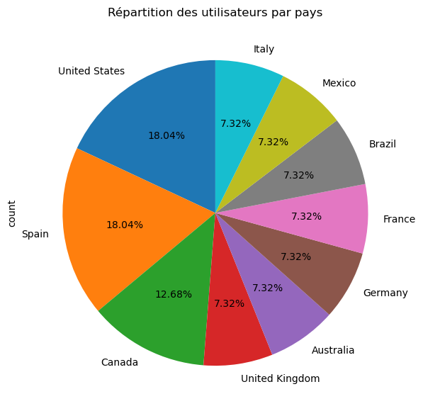
1.2 Modification des données
User ID est une colonne qui ne sert pas à grand chose, on peut la supprimer.
filtre = ['United Kingdom', 'Germany', 'France', 'Spain', 'Italy']

# mask =  (df_complet['Country'] in filtre) # erreur
# mask = df_complet['Country']==filtre[0] | df_complet['Country']==filtre[1] | df_complet['Country']==filtre[2] | df_complet['Country']==filtre[3] | df_complet['Country']==filtre[4] # erreur
mask = df_complet['Country'].isin(filtre)
df = df_complet[mask]
df| Subscription Type | Monthly Revenue | Join Date | Last Payment Date | Country | Age | Gender | Device | Plan Duration | |
|---|---|---|---|---|---|---|---|---|---|
| 2 | Standard | 12 | 28-02-23 | 27-06-23 | United Kingdom | 42 | Male | Smart TV | 1 Month |
| 4 | Basic | 10 | 01-05-23 | 28-06-23 | Germany | 33 | Male | Smartphone | 1 Month |
| 5 | Premium | 15 | 18-03-22 | 27-06-23 | France | 29 | Female | Smart TV | 1 Month |
| 8 | Standard | 12 | 20-10-22 | 23-06-23 | Spain | 37 | Male | Smartphone | 1 Month |
| 9 | Premium | 15 | 07-01-23 | 22-06-23 | Italy | 44 | Female | Smart TV | 1 Month |
| ... | ... | ... | ... | ... | ... | ... | ... | ... | ... |
| 2490 | Premium | 13 | 18-07-22 | 11-07-23 | France | 41 | Female | Smartphone | 1 Month |
| 2493 | Premium | 12 | 21-07-22 | 15-07-23 | Spain | 36 | Male | Smart TV | 1 Month |
| 2494 | Basic | 15 | 23-07-22 | 12-07-23 | Italy | 43 | Female | Laptop | 1 Month |
| 2495 | Premium | 14 | 25-07-22 | 12-07-23 | Spain | 28 | Female | Smart TV | 1 Month |
| 2496 | Basic | 15 | 04-08-22 | 14-07-23 | Spain | 33 | Female | Smart TV | 1 Month |
1183 rows × 9 columns
1.3 Aggregations/Visualisations
Nombre d’utilisateurs par pays
pd.DataFrame({  'Nombre': df['Country'].value_counts(),
                'Pourcentage (%)': df['Country'].value_counts(normalize=True)
})| Nombre | Pourcentage (%) | |
|---|---|---|
| Country | ||
| Spain | 451 | 0.381234 |
| United Kingdom | 183 | 0.154691 |
| Germany | 183 | 0.154691 |
| France | 183 | 0.154691 |
| Italy | 183 | 0.154691 |
df['Country'].value_counts().plot(kind='pie', autopct='%1.2f%%', legend=False)
plt.title('Répartition des utilisateurs par pays')
plt.show()

# sns.countplot(data=df, x='Country');

# px.pie(df,
#      names='Country',
#      title='Répartition des utilisateurs par pays'
#      ).update_traces(texttemplate='%{label}<br>%{value}<br>%{percent:.2%}',
#                      textposition='outside').show()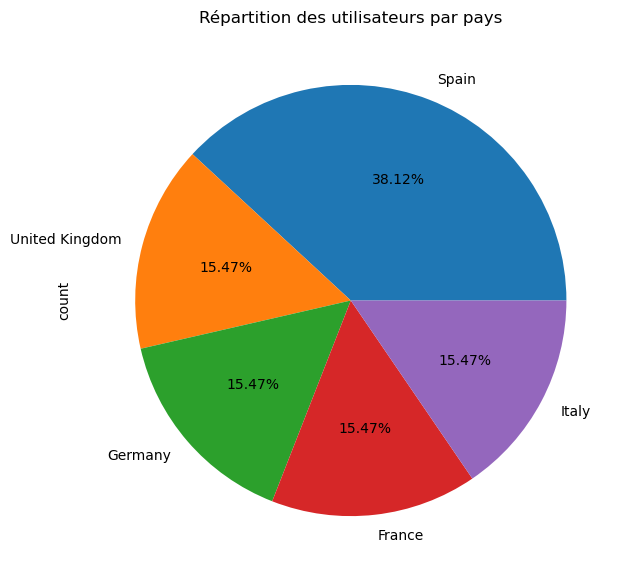
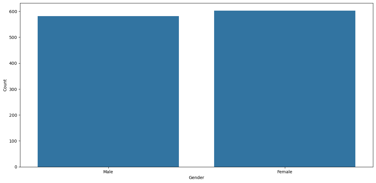
Nombre d’utilisateurs par sexe
pd.DataFrame({  'Nombre': df['Gender'].value_counts(),
                'Pourcentage (%)': df['Gender'].value_counts(normalize=True)
})| Nombre | Pourcentage (%) | |
|---|---|---|
| Gender | ||
| Female | 602 | 0.508876 |
| Male | 581 | 0.491124 |
df['Gender'].value_counts().plot(kind='pie', autopct='%1.2f%%', legend=False)
plt.title('Répartition des utilisateurs par sexe')
plt.show()

# sns.countplot(data=df, x='Gender')
# plt.xlabel('Gender')
# plt.ylabel('Count');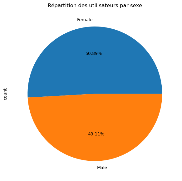
Nombre d’utilisateurs par age
pd.DataFrame({  'Nombre': df['Age'].value_counts(),
                'Pourcentage (%)': df['Age'].value_counts(normalize=True)
})| Nombre | Pourcentage (%) | |
|---|---|---|
| Age | ||
| 31 | 60 | 0.050719 |
| 41 | 58 | 0.049028 |
| 28 | 58 | 0.049028 |
| 46 | 53 | 0.044801 |
| 49 | 52 | 0.043956 |
| 30 | 51 | 0.043111 |
| 51 | 50 | 0.042265 |
| 35 | 50 | 0.042265 |
| 42 | 50 | 0.042265 |
| 37 | 49 | 0.041420 |
| 39 | 49 | 0.041420 |
| 36 | 48 | 0.040575 |
| 47 | 46 | 0.038884 |
| 32 | 45 | 0.038039 |
| 33 | 45 | 0.038039 |
| 38 | 45 | 0.038039 |
| 43 | 45 | 0.038039 |
| 34 | 45 | 0.038039 |
| 40 | 44 | 0.037194 |
| 45 | 43 | 0.036348 |
| 44 | 43 | 0.036348 |
| 48 | 41 | 0.034658 |
| 29 | 39 | 0.032967 |
| 27 | 37 | 0.031276 |
| 50 | 37 | 0.031276 |
Nombre d’utilisateurs par device
pd.DataFrame({  'Nombre': df['Device'].value_counts(),
                'Pourcentage (%)': df['Device'].value_counts(normalize=True)
})| Nombre | Pourcentage (%) | |
|---|---|---|
| Device | ||
| Laptop | 316 | 0.267117 |
| Smart TV | 297 | 0.251057 |
| Smartphone | 286 | 0.241758 |
| Tablet | 284 | 0.240068 |
df['Device'].value_counts().plot(kind='pie', autopct='%1.2f%%', legend=False)
plt.title('Répartition des utilisateurs par type d\'appareil')
plt.show()

# sns.countplot(data=df, x='Device')
# plt.xlabel('Device')
# plt.ylabel('Count')
# plt.show()

# px.pie(df,
#      names='Device',
#      title='Répartition des utilisateurs par type d\'appareil'
#      ).update_traces(texttemplate='%{label}<br>%{value}<br>%{percent:.2%}',
# textposition='outside').show() 
Répartition des utilisateurs par type d’abonnement
pd.DataFrame({  'Nombre': df['Subscription Type'].value_counts(),
                'Pourcentage (%)': df['Subscription Type'].value_counts(normalize=True)
})| Nombre | Pourcentage (%) | |
|---|---|---|
| Subscription Type | ||
| Basic | 474 | 0.400676 |
| Premium | 366 | 0.309383 |
| Standard | 343 | 0.289941 |
df['Subscription Type'].value_counts().plot(kind='pie', autopct='%1.1f%%')
plt.title("Répartition des utilisateurs par type d'abonnement")
plt.show()

px.pie(df,
     names='Subscription Type',
     title="Répartition des utilisateurs par type d'abonnement"
     ).update_traces(texttemplate='%{label}<br>%{value}<br>%{percent:.2%}',
                     textposition='outside').show()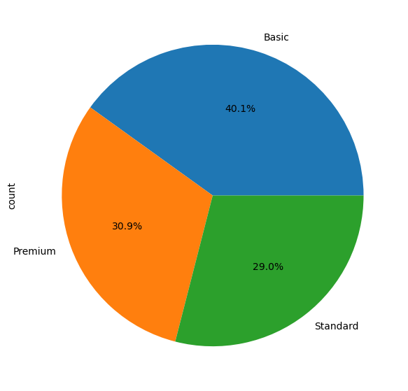
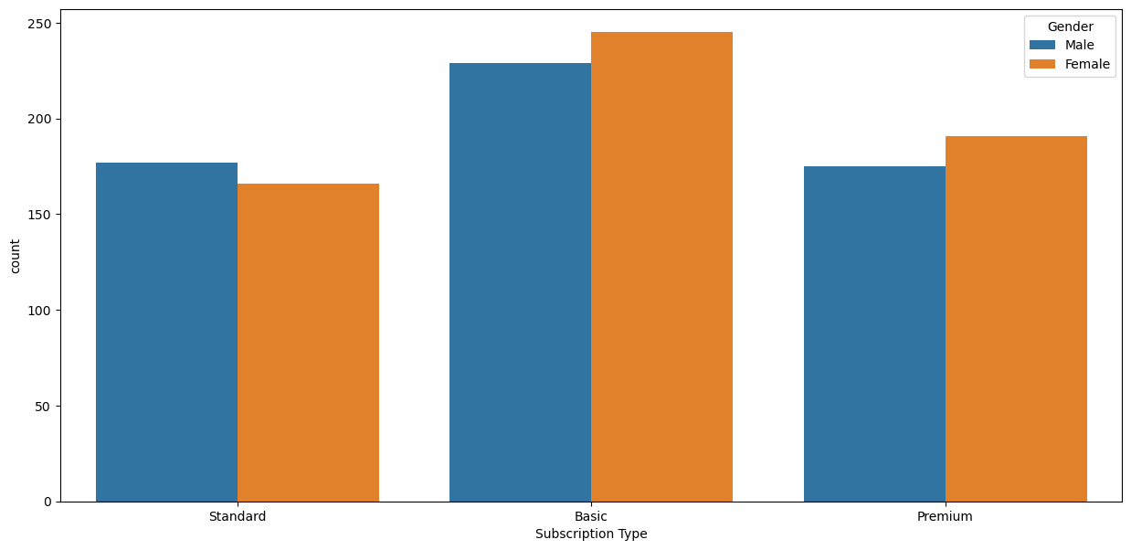
Unable to display output for mime type(s): application/vnd.plotly.v1+jsonNombre d’utilisateurs par type d’abonnement et genre
# pd.crosstab(df['Subscription Type'], df['Gender']) # tableau de contingence
# pd.crosstab(df['Subscription Type'], df['Gender'], normalize='index') # pourcentage par ligne
# pd.crosstab(df['Subscription Type'], df['Gender'], normalize='columns') # pourcentage par colonne
pd.crosstab(df['Subscription Type'], df['Gender'], normalize='all') # pourcentage total| Gender | Female | Male |
|---|---|---|
| Subscription Type | ||
| Basic | 0.207101 | 0.193576 |
| Premium | 0.161454 | 0.147929 |
| Standard | 0.140321 | 0.149620 |
Type d’abonnement par pays, genre et device
pd.pivot_table(df, index='Country', columns=['Gender','Device'], values='Subscription Type', aggfunc='count')| Gender | Female | Male | ||||||
|---|---|---|---|---|---|---|---|---|
| Device | Laptop | Smart TV | Smartphone | Tablet | Laptop | Smart TV | Smartphone | Tablet |
| Country | ||||||||
| France | 29 | 25 | 24 | 13 | 23 | 18 | 23 | 28 |
| Germany | 27 | 26 | 17 | 24 | 36 | 16 | 19 | 18 |
| Italy | 20 | 31 | 20 | 20 | 30 | 15 | 27 | 20 |
| Spain | 56 | 63 | 49 | 65 | 51 | 63 | 53 | 51 |
| United Kingdom | 22 | 16 | 27 | 28 | 22 | 24 | 27 | 17 |
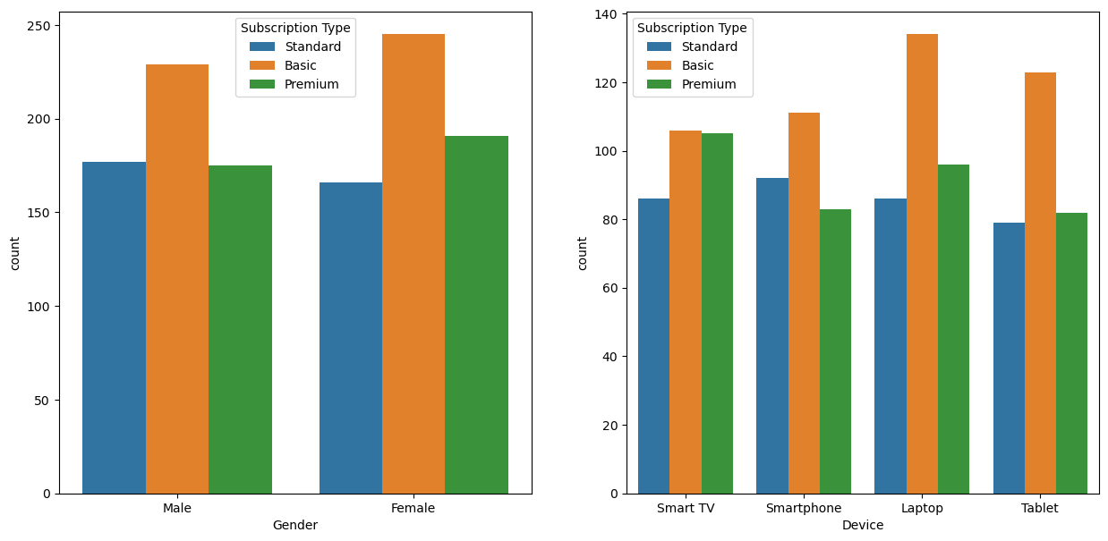
Type d’abonnement par pays et genre
for i,c in enumerate(['Gender','Device']):
    plt.subplot(1,2,i+1)
    sns.countplot(data=df, x=c, hue='Subscription Type');